Chapter 10 - Parametric and Polar Curves

Parametric curves

Videos

Review Videos

Videos, Organic Chemistry Tutor

• Intro to parametric equations and graphing

Link to original

Theory

Theory 1

Parametric curves are curves traced by the path of a ‘moving’ point. An independent parameter, such as $t$ for ‘time’, controls both $x$ and $y$ values through Cartesian coordinate functions $x(t)$ and $y(t)$. The coordinates of the moving point are $(x(t),y(t))$.

Parametric curve

A parametric curve is a function from parameter space $\mathbb{R}$ to the plane ${\mathbb{R}}^2$ given in terms of coordinate functions:

$$t⟼(x(t),y(t))$$

Other notations

Be aware that sometimes the coordinate functions are written with $f$ and $g$ (or yet other letters) like this:

$$(x,y)=(f(t),g(t))$$

Or simply equating coordinate letters with functions: $x=f(t),y=g(t)$

Sometimes a different parameter is used, like $s$ or $u$.

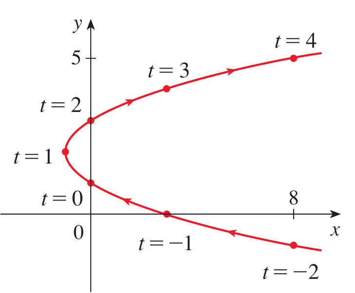
For example, suppose:

$$x=t^2-2t,y=t+1$$

The curve traced out is a parabola that opens horizontally:

---

Given a parametric curve, we can create an equation satisfied by $x$ and $y$ variables by solving for $t$ in either coordinate function (inverting either $f$ or $g$) and plugging the result into the other function.

In the example:

$$\begin{array}{c}y=t+1\gg \gg t=y-1\\ \\ \gg \gg x=t^2-2t\gg \gg x=(y-1{)}^2-2(y-1)\\ \\ \gg \gg x=y^2-4y+3\gg \gg x=(y-2{)}^2-1\end{array}$$

This is the equation of a parabola centered at $(-1,2)$ that opens to the right.

Image of a parametric curve

The image of a parametric curve is the set of output points $(x(t),y(t))$ that are traversed by the moving point.

A parametric curve has hidden information that isn’t contained in the image:

• The time values $t$ when the moving point is found in various locations.
• The speed at which the curve is traversed.
• The direction in which the curve is traversed.

---

We can reparametrize a parametric curve to use a different parameter or different coordinate functions while leaving the image unchanged.

In the previous example, shift $t$ by $1$:

$$\begin{array}{c}x=(t+1{)}^2-2(t+1),y=(t+1)+1\\ \\ \gg \gg x=t^2-1,y=t+2\end{array}$$

Since the parameter $t$ and the parameter $t+1$ both cover the same values for $t\in (-\infty ,\infty )$, the same curve is traversed. But the moving point in the second, shifted version reaches any given location one unit earlier in time. (When $t=-1$ in the second version, the input to $x(t)$ and $y(t)$ is the same as when $t=0$ in the first one.)

Link to original

Illustration

Example - Parametric circles

Parametric circles

The standard equation of a circle of radius $R$ centered at the point $(h,k)$:

$$(x-h{)}^2+(y-k{)}^2=R^2$$

This equation says that the distance from a point $(x,y)$ on the circle to the center point $(h,k)$ equals $R$. This fact defines the circle.

Parametric coordinates for the circle:

$$x=h+R\cos t,y=k+R\sin t,t\in [0,2\pi )$$

For example, the unit circle $x^2+y^2=1$ is parametrized by $x=\cos t$ and $y=\sin t$.

Link to original

Example - Parametric lines

Parametric lines

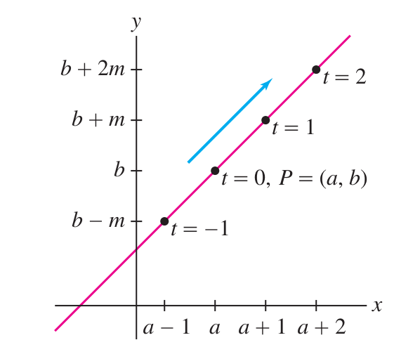
(1) Parametric coordinate functions for a line:

$$x=a+rt,y=b+st,t\in (-\infty ,+\infty )$$

Compare this to the graph of linear function:

$$y=mx+b\text{some }m,b$$

Vertical lines cannot be described as the graph of a function. We must use $x=a$.

---

(2) Parametric lines can describe all lines equally well, including horizontal and vertical lines.

A vertical line $x=a$ is achieved by setting $s=0$ and $r\ne 0$.

A horizontal line $y=b$ is achieved by setting $r=0$ and $s\ne 0$.

A non-vertical line $y=mx+b$ may be achieved by setting $s=m$ and $r=1$, and $a=0$.

---

(3) Assuming that $r\ne 0$, the parametric coordinate functions describe a line satisfying:

$$\begin{array}{c}y=b+s\left(\frac{x-a}{r}\right)\\ \\ \gg \gg y=\frac{s}{r}\cdot x+\left(b-\frac{s}{r}\cdot a\right)\end{array}$$

and therefore the slope is $m=\frac{s}{r}$ and the $y$-intercept is $b-\frac{s}{r}\cdot a$.

---

(4) The point-slope construction of a line has a parametric analogue:

$$\begin{array}{c}\text{point-slope line:}\\ \\ y-a=m(x-b)(x,y)=(a+t,b+mt)\end{array}$$

Link to original

Example - Parametric ellipses

Parametric ellipses

The general equation of an ellipse centered at $(h,k)$ with half-axes $a$ and $b$ is:

$${\left(\frac{x-h}{a}\right)}^2+{\left(\frac{y-k}{b}\right)}^2=1$$

This equation represents a stretched unit circle:

• by $a$ in the $x$-axis
• by $b$ in the $y$-axis

Parametric coordinate functions for the general ellipse:

$$x=h+a\cos t,y=k+b\sin t,t\in [0,2\pi )$$ Link to original

Example - Parametric cycloids

Parametric cycloids

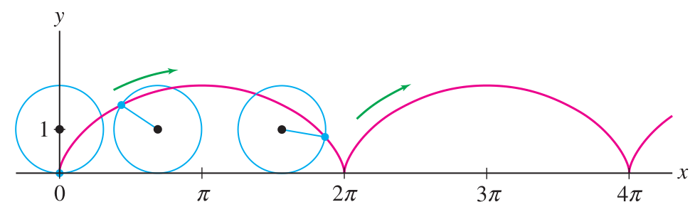
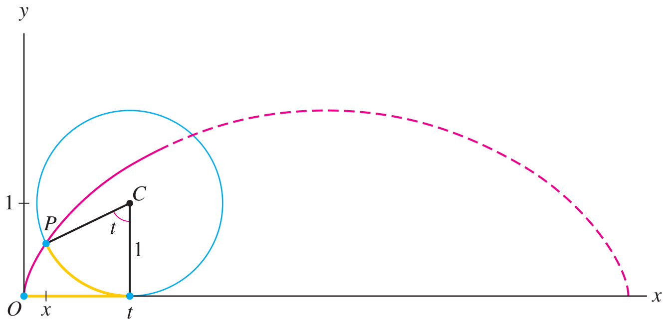
The cycloid is the curve traced by a pen attached to the rim of a wheel as it rolls.

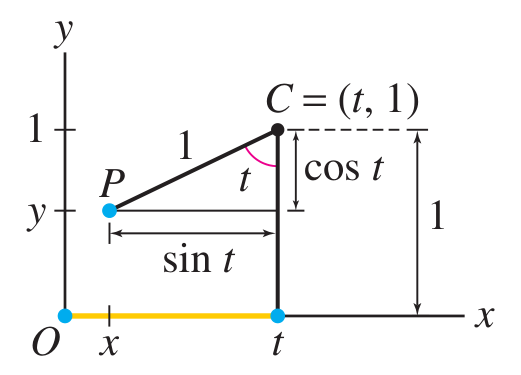
It is easy to describe the cycloid parametrically. Consider the geometry of the situation:

The center $C$ of the wheel is moving rightwards at a constant speed of $1$, so its position is $(t,1)$. The angle is revolving at the same constant rate of $1$ (in radians) because the radius is $1$.

The triangle shown has base $\sin t$, so the $x$ coordinate is $t-\sin t$. The $y$ coordinate is $1-\cos t$.

So the coordinates of the point $P=(x,y)$ are given parametrically by:

$$x=t-\sin t,y=1-\cos t,t>0$$

If the circle has another radius, say $R$, then the parametric formulas change to:

$$x=Rt-R\sin t,y=R-R\cos t,t>0$$Link to original

Calculus with parametric curves

Theory - Slope, concavity

Theory 1

We can use $x(t)$ and $y(t)$ data to compute the slope of a parametric curve in terms of $t$.

Slope formula

Given a parametric curve $(x(t),y(t))$, its slope satisfies:

$$\frac{dy}{dx}=\frac{y^{\prime }(t)}{x^{\prime }(t)}(\text{where }{x}^{\prime }(t)\ne 0)$$

Concavity formula

Given a parametric curve $(x(t),y(t))$, its concavity satisfies the formula:

$$\frac{d^{2}y}{d{x}^2}=\frac{d}{dt}\left(\frac{y^{\prime }(t)}{x^{\prime }(t)}\right)\cdot \frac{1}{x^{\prime }(t)}(\text{where }{x}^{\prime }(t)\ne 0)$$

Extra - Derivation of slope and concavity formulas

For both derivations, it is necessary to view $t$ as a function of $x$ through the inverse parameter function. For example if $x=f(t)$ is the parametrization, then $t=f^{-1}(x)$ is the inverse parameter function.

We will need the derivative $\frac{dt}{dx}$ in terms of $t$. For this we use the formula for derivative of inverse functions:

$$\frac{dt}{dx}=\frac{1}{\frac{dx}{dt}}$$

Given all this, both formulas are simple applications of the chain rule.

For the slope:

$$\begin{array}{c}\frac{dy}{dx}=\frac{dy}{dt}\cdot \frac{dt}{dx}\gg \gg y^{\prime }(t)\cdot \frac{1}{dx/dt}\\ \\ \gg \gg \frac{y^{\prime }(t)}{x^{\prime }(t)}\end{array}$$

For the concavity:

$$\begin{array}{c}\frac{d^{2}y}{d{x}^2}=\frac{d}{dx}\left(\frac{dy}{dx}\right)\gg \gg \frac{d}{dt}\left(\frac{dy}{dx}\right)\cdot \frac{dt}{dx}\\ \\ \gg \gg \frac{d}{dt}\left(\frac{y^{\prime }(t)}{x^{\prime }(t)}\right)\cdot \frac{1}{x^{\prime }(t)}\end{array}$$

(In the second step we inserted the formula for $\frac{dy}{dx}$ from the slope.)

---

Pure vertical, Pure horizontal movement

In view of the formula $\frac{dy}{dx}=\frac{y^{\prime }(t)}{x^{\prime }(t)}$, we see:

• Pure vertical: when $x^{\prime }(t)=0$ and yet $y^{\prime }(t)\ne 0$
• Pure horizontal: when $y^{\prime }(t)=0$ and yet $x^{\prime }(t)\ne 0$

When $x^{\prime }(t_0)=y^{\prime }(t_0)=0$ for the same $t=t_0$, we have a stationary point, which might subsequently progress into pure vertical, pure horizontal, or neither.

Link to original

Illustration

Example - Tangent to a cycloid

Tangent to a cycloid

Find the tangent line (described parametrically) to the cycloid $(4t-4\sin t,4-4\cos t)$ when $t=\pi /4$.

Solution

(1) Compute $x^{\prime }$ and $y^{\prime }$.

Find $x^{\prime }(t)$ and $y^{\prime }(t)$:

$$\begin{array}{rl}x(t)& =4t-4\sin t\gg \gg x^{\prime }(t)=4-4\cos t\\ & \\ y(t)& =4-4\cos t\gg \gg y^{\prime }(t)=4\sin t\end{array}$$

---

(2) Plug in $t=\pi /4$:

$$\begin{array}{c}{x}^{\prime }(\pi /4)\gg \gg 4-4\cos (\pi /4)\gg \gg 4-2\sqrt{2}\\ \\ y^{\prime }(\pi /4)\gg \gg 4\sin (\pi /4)\gg \gg 2\sqrt{2}\end{array}$$

---

(3) Apply formula: $\frac{dy}{dx}=\frac{y^{\prime }}{x^{\prime }}$:

Calculate $\frac{dy}{dx}$ at $t=\pi /4$:

$$\begin{array}{c}\frac{dy}{dx}(\pi /4)=\frac{y^{\prime }(\pi /4)}{x^{\prime }(\pi /4)}\gg \gg \frac{2\sqrt{2}}{4-2\sqrt{2}}\\ \\ \gg \gg \frac{2\sqrt{2}}{4-2\sqrt{2}}\cdot \frac{4+2\sqrt{2}}{4+2\sqrt{2}}\\ \\ \gg \gg \frac{8\sqrt{2}+8}{16-8}\gg \gg \sqrt{2}+1\end{array}$$

So:

$${\frac{dy}{dx}|}_{t=\pi /4}=\sqrt{2}+1$$

This is the slope $m$ for our line.

---

(4) Need the point $P$ for our line. Find $(x,y)$ at $t=\pi /4$.

Plug $t=\pi /4$ into parametric formulas:

$$\begin{array}{c}(x(t),y(t)){|}_{t=\pi /4}\gg \gg \left(4\frac{\pi }{4}-4\sin (\pi /4),4-4\cos (\pi /4)\right)\\ \\ \gg \gg \left(\pi -2\sqrt{2},4-2\sqrt{2}\right)\end{array}$$

---

(5) Point-slope formulation of tangent line:

$$x=a+t,y=b+mt$$

Inserting data:

$$x=(\pi -2\sqrt{2})+t,y=(4-2\sqrt{2})+(\sqrt{2}+1)t$$ Link to original

Example - Vertical and horizontal tangents of the circle

Vertical and horizontal tangents of the circle

Consider the circle parametrized by $x=\cos t$ and $y=\sin t$. Find the points where the tangent lines are vertical or horizontal.

Solution

(1) For the points with vertical tangent line, we find where the moving point has $x^{\prime }(t)=0$ (purely vertical motion):

$$\begin{array}{c}{x}^{\prime }(t)=-\sin t,\\ \\ x^{\prime }(t)=0\gg \gg -\sin t=0\\ \\ \gg \gg t=0,\pi \end{array}$$

The moving point is at $(1,0)$ when $t=0$, and at $(-1,0)$ when $t=\pi$.

---

(2) For the points with horizontal tangent line, we find where the moving point has $y^{\prime }(t)=0$ (purely horizontal motion):

$$\begin{array}{c}{y}^{\prime }(t)=\cos t,\\ \\ y^{\prime }(t)=0\gg \gg \cos t=0\\ \\ \gg \gg t=\frac{\pi }{2},\frac{3\pi }{2}\end{array}$$

The moving point is at $(0,1)$ when $t=\pi /2$, and at $(0,-1)$ when $t=3\pi /2$.

Link to original

Example - Finding the point with specified slope

Finding the point with specified slope

Consider the parametric curve given by $(x,y)=(t^2,t^3)$. Find the point where the slope of the tangent line to this curve equals 5.

Solution

(1) Compute the derivatives:

$$x^{\prime }(t)=2t,y^{\prime }(t)=3t^2$$

Therefore the slope of the tangent line, in terms of $t$:

$$\begin{array}{c}m=\frac{dy}{dx}=\frac{y^{\prime }(t)}{x^{\prime }(t)}\\ \\ \gg \gg \frac{3t^2}{2t}\gg \gg \frac{3}{2}t\end{array}$$

---

(2) Set up equation:

$$\begin{array}{c}m=5\\ \\ \frac{3}{2}t=5\\ \\ \gg \gg t=\frac{10}{3}\end{array}$$

---

(3) Find the point:

$$(x,y){|}_{t=10/3}\gg \gg \left(\frac{100}{9},\frac{1000}{27}\right)$$ Link to original

More calculus with parametric curves

Theory - Arclength

Theory 2

Arclength formula

The arclength of a parametric curve with coordinate functions $x(t)$ and $y(t)$ is:

$$L={\int }_a^b\sqrt{(x^{\prime }{)}^2+(y^{\prime }{)}^2}dt$$

This formula assumes the curve is traversed one time as $t$ increases from $a$ to $b$.

Counts total traversal

This formula applies when the curve image is traversed one time by the moving point.

Sometimes a parametric curve traverses its image with repetitions. The arclength formula would add length from each repetition!

Extra - Derivation of arclength formula

The arclength of a parametric curve is calculated by integrating the infinitesimal arc element:

$$\begin{array}{c}ds=\sqrt{d{x}^2+d{y}^2}\\ \\ L={\int }_a^{b}ds\end{array}$$

In order to integrate $ds$ in the $t$ variable, as we must for parametric curves, we convert $ds$ to a function of $t$:

$$\begin{array}{c}ds=\sqrt{d{x}^2+d{y}^2}\gg \gg \sqrt{\frac{1}{d{t}^2}\cdot \left(d{x}^2+d{y}^2\right)\cdot d{t}^2}\\ \\ \gg \gg \sqrt{\frac{d{x}^2}{d{t}^2}+\frac{d{y}^2}{d{t}^2}}\cdot \sqrt{d{t}^2}\gg \gg \sqrt{{\left(\frac{dx}{dt}\right)}^2+{\left(\frac{dy}{dt}\right)}^2}dt\\ \\ \gg \gg ds=\sqrt{x^{\prime }(t{)}^2+y^{\prime }(t{)}^2}dt\end{array}$$

So we obtain $ds=\sqrt{(x^{\prime }{)}^2+(y^{\prime }{)}^2}dt$ and the arclength formula follows from this:

$$L={\int }_a^b\sqrt{(x^{\prime }{)}^2+(y^{\prime }{)}^2}dt$$

Link to original

Illustration

Example - Perimeter of a circles

Perimeter of a circle

(1) The perimeter of the circle $(R\cos t,R\sin t)$ is easily found. We have $(x^{\prime },y^{\prime })=(-R\sin t,R\cos t)$, and therefore:

$$\begin{array}{c}(x^{\prime }{)}^2+(y^{\prime }{)}^2=(-R\sin t{)}^2+(R\cos t{)}^2\\ \\ \gg \gg R^2{\sin }^{2}t+R^2{\cos }^{2}t\gg \gg R^2\\ \\ ds=\sqrt{(x^{\prime }{)}^2+(y^{\prime }{)}^2}dt=Rdt\end{array}$$

---

(2) Integrate around the circle:

$$\begin{array}{c}\text{Perimeter}={\int }_0^{2\pi }ds\gg \gg {\int }_0^{2\pi }Rdt\\ \\ \gg \gg Rt{|}_0^{2\pi }=2\pi R\end{array}$$ Link to original

Example - Perimeter of an asteroid

Perimeter of an asteroid

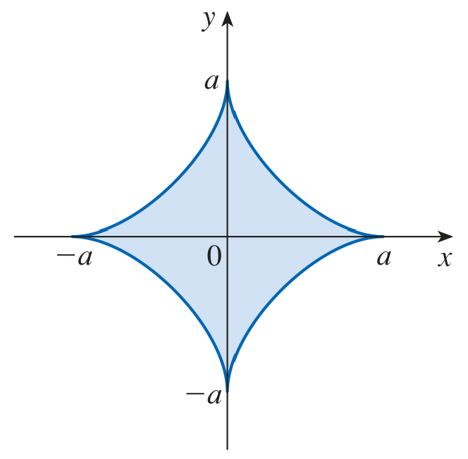
Find the perimeter length of the ‘asteroid’ given parametrically by $(x,y)=\left(a{\cos }^3\theta ,a{\sin }^3\theta \right)$ for $a=2$.

Solution

(1) Notice: Throughout this problem we use the parameter $\theta$ instead of $t$. This does not mean we are using polar coordinates!

Compute the derivatives in $\theta$:

$$\left(x^{\prime },y^{\prime }\right)=\left(3a{\cos }^2\theta \sin \theta ,3a{\sin }^2\theta \cos \theta \right)$$

---

(2) Compute the infinitesimal arc element.

$$\begin{array}{c}(x^{\prime }{)}^2+(y^{\prime }{)}^2\gg \gg 9a^2{\cos }^4\theta {\sin }^2\theta +9a^2{\sin }^4\theta {\cos }^2\theta \\ \\ \gg \gg 9a^2{\sin }^2\theta {\cos }^2\theta \left({\cos }^2\theta +{\sin }^2\theta \right)\\ \\ \gg \gg 9a^2{\sin }^2\theta {\cos }^2\theta \end{array}$$

Plug into the arc element, simplify:

$$\begin{array}{c}ds=\sqrt{(x^{\prime }{)}^2+y^{\prime }{)}^2}d\theta \\ \\ \gg \gg \sqrt{9a^2{\sin }^2\theta {\cos }^2\theta }d\theta \\ \\ \gg \gg ds=3a\left|\sin \theta \cos \theta \right|d\theta \end{array}$$

---

(3) Bounds of integration?

Easiest to use $\theta \in [0,\pi /2]$. This covers one edge of the asteroid. Then multiply by 4 for the final answer.

On the interval $\theta \in [0,\pi /2]$, the factor $3a\sin \theta \cos \theta$ is positive. So we can drop the absolute value and integrate directly.

Absolute values matter!

If we tried to integrate on the whole range $\theta \in [0,2\pi ]$, then $3a\sin \theta \cos \theta$ really does change sign.

To perform integration properly with these absolute values, we’d need to convert to a piecewise function by adding appropriate minus signs.

---

(4) Integrate the arc element:

$$\begin{array}{c}{\int }_0^{\pi /2}ds\gg \gg {\int }_0^{\pi /2}3a\sin \theta \cos \theta d\theta \\ \\ \gg \gg 3a{\int }_{u=0}^{1}udu\\ \\ \gg \gg 3a{\frac{u^2}{2}|}_0^1\gg \gg \frac{3a}{2}\end{array}\text{\hspace{1em}(u=sinθ)}$$

Finally, multiply by 4 to get the total perimeter: $L=6a$

Link to original

Theory - Distance, speed

Theory 3

Distance function

The distance function $s(t)$ returns the total distance traveled by the particle from a chosen starting time $t_0$ up to the (input) time $t$:

$$s(t)={\int }_{t_0}^{t}ds={\int }_{t_0}^t\sqrt{x^{\prime }(u{)}^2+y^{\prime }(u{)}^2}du$$

We need the dummy variable $u$ so that the integration process does not conflict with $t$ in the upper bound.

---

Speed function

The speed of a moving particle is the rate of change of distance:

$$v(t)=s^{\prime }(t)=\sqrt{x^{\prime }(t{)}^2+y^{\prime }(t{)}^2}$$

This formula can be explained in either of two ways:

1. Apply the Fundamental Theorem of Calculus to the integral formula for $s(t)$.
2. Consider $ds=\sqrt{x^{\prime }(t{)}^2+y^{\prime }(t{)}^2}dt$ for a small change $dt$: so the rate of change of arclength is $\frac{ds}{dt}$, in other words $s^{\prime }(t)$.

Link to original

Illustration

Example - Speed, distance, displacement

Speed, distance, displacement

The parametric curve $\left(t,\frac{2}{3}{t}^{3/2}\right)$ describes the position of a moving particle ($t$ measuring seconds).
(a) What is the speed function?

Suppose the particle travels for $8$ seconds starting at $t=0$.
(b) What is the total distance traveled?
(c) What is the total displacement?

Solution

(a)

Compute derivatives:

$$\left(x^{\prime },y^{\prime }\right)=\left(1,t^{1/2}\right)$$

Now compute the speed:

$$\begin{gathered} (x^{\prime }{)}^2+(y^{\prime }{)}^2=1+(t^{1/2}{)}^2=1+t \\ \gg \gg v(t)=\sqrt{(x^{\prime }{)}^2+(y^{\prime }{)}^2}=\sqrt{1+t} \end{gathered}$$

---

(b)

Distance traveled by using speed.

Compute total distance traveled function:

$$s(t)={\int }_{u=0}^t\sqrt{1+u}du$$

Substitute $w=1+u$ and $dw=du$. New bounds are $1$ and $1+t$. Calculate:

$$\begin{array}{c}\gg \gg {\int }_1^{1+t}\sqrt{w}dw\\ \\ \gg \gg \frac{2}{3}{w}^{3/2}{|}_1^{1+t}\gg \gg \frac{2}{3}\left((1+t{)}^{3/2}-1\right)\end{array}$$

The distance traveled up to $t=8$ is:

$$s(8)=\frac{2}{3}\left(9^{3/2}-1\right)\gg \gg \frac{2}{3}(27-1)\gg \gg \frac{52}{3}$$

---

(c)

Displacement formula: $d=\sqrt{(x_1-x_0{)}^2+(y_1-y_0{)}^2}$

Now compute starting and ending points.

For starting point, insert $t=0$:

$$(x(t),y(t)){|}_{t=0}\gg \gg \left(t,\frac{2}{3}{t}^{3/2}\right){|}_{t=0}\gg \gg (0,0)$$

For ending point, insert $t=8$:

$$\begin{array}{c}(x(t),y(t)){|}_{t=8}\gg \gg \left(t,\frac{2}{3}{t}^{3/2}\right){|}_{t=8}\\ \\ \gg \gg \left(8,\frac{2}{3}{8}^{3/2}\right)\gg \gg \left(8,\frac{32\sqrt{2}}{3}\right)\end{array}$$

Insert $(0,0)$ and $\left(8,32\sqrt{2}/3\right)$:

$$\begin{array}{c}\gg \gg \sqrt{8^2+{\left(\frac{32\sqrt{2}}{3}\right)}^2}\gg \gg \sqrt{64+\frac{2048}{9}}\\ \\ \gg \gg \frac{\sqrt{2624}}{3}\end{array}$$ Link to original

Theory - Surface area of revolutions

Theory 4

Surface area of a surface of revolution: thin bands

Suppose a parametric curve $(x(t),y(t))$ is revolved around the $x$-axis or the $y$-axis.

The surface area is:

$$A={\int }_a^{b}2\pi R(t)\sqrt{(x^{\prime }{)}^2+(y^{\prime }{)}^2}dt$$

The radius $R(t)$ should be the distance to the axis:

$$\begin{array}{rl}R(t)& =y(t)\text{revolution about x-axis}\\ R(t)& =x(t)\text{revolution about y-axis}\end{array}$$

This formulas adds the areas of thin bands, but the bands are demarcated using parametric functions instead of input values of a graphed function.

The formula assumes that the curve is traversed one time as $t$ increases from $a$ to $b$.

Link to original

Illustration

Example - Surface of revolution - parametric circle

Surface of revolution - parametric circle

By revolving the unit upper semicircle about the $x$-axis, we can compute the surface area of the unit sphere.

Parametrization of the unit upper semicircle:

$$\begin{array}{c}(x,y)=(\cos t,\sin t)\\ \\ \gg \gg (x^{\prime },y^{\prime })=(-\sin t,\cos t)\end{array}$$

---

Therefore, the arc element:

$$\begin{array}{c}ds=\sqrt{(x^{\prime }{)}^2+(y^{\prime }{)}^2}dt\\ \\ \gg \gg \sqrt{(-\sin t{)}^2+(\cos t{)}^2}dt\gg \gg dt\end{array}$$

Now for $R(t)$ we choose $R(t)=y(t)=\sin t$ because we are revolving about the $x$-axis.

---

Plugging all this into the integral formula and evaluating gives:

$$A={\int }_0^{\pi }2\pi \sin tdt\gg \gg -2\pi \cos t{|}_0^{\pi }\gg \gg 4\pi$$

Notice: This method is a little easier than the method using the graph $y=\sqrt{1-x^2}$.

Link to original

Example - Surface of revolution - parametric curve

Surface of revolution - parametric curve

Set up the integral which computes the surface area of the surface generated by revolving about the $x$-axis the curve $(t^3,t^2-1)$ for $0\le t\le 1$.

Solution

For revolution about the $x$-axis, we set $R=y(t)=t^2-1$.

Then compute $ds$:

$$\begin{array}{c}ds=\sqrt{(x^{\prime }{)}^2+(y^{\prime }{)}^2}\gg \gg \sqrt{(3t^2{)}^2+(2t{)}^2}\gg \gg \sqrt{9t^4+4t^2}\\ \\ \gg \gg \sqrt{t^2(9t^2+4)}\gg \gg t\sqrt{9t^2+4}\end{array}$$

Therefore the desired integral is:

$$A={\int }_0^{1}2\pi Rds\gg \gg {\int }_0^{1}2\pi (t^2-1)t\sqrt{9t^2+4}dt$$Link to original

Polar curves

Videos

Review Videos

Videos, Organic Chemistry Tutor

• Polar coordinates intro
• Graphing polar curves

Link to original

Theory - Polar points, polar curves

Theory 1

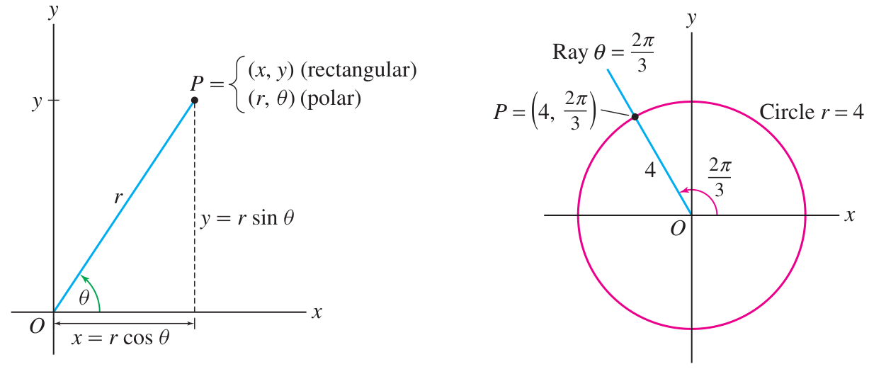
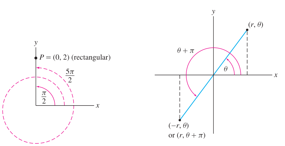
Polar coordinates are pairs of numbers $(r,\theta )$ which identify points in the plane in terms of distance to origin and angle from $+x$-axis:

Converting $\mathrm{Polar}\leftrightarrow \mathrm{Cartesian}$

$$\begin{array}{l}\text{Polar}\to \text{Cartesian}\\ x=r\cos \theta \\ y=r\sin \theta \end{array}\begin{array}{l}\text{Cartesian}\to \text{Polar}\\ r=\sqrt{x^2+y^2}\\ \tan \theta =\frac{y}{x}(x\ne 0)\end{array}$$

---

Polar coordinates have many redundancies: unlike Cartesian which are unique!

• For example: $(r,\theta )=(r,\theta +2\pi )$
  • And therefore also $(r,\theta )=(r,\theta -2\pi )$ (negative $\theta$ can happen)
• For example: $(-r,\theta )=(r,\theta +\pi )$ for every $r,\theta$
• For example: $(0,\theta )=(0,0)$ for any $\theta$

Polar coordinates cannot be added: they are not vector components!

• For example $(5,\pi /3)+(2,\pi /6)\ne (7,\pi /2)$
• Whereas Cartesian coordinates can be added: $(1,4)+(2,-2)=(3,2)$

---

The transition formulas $\text{Cartesian}\to \text{Polar}$ require careful choice of $\theta$.

• The standard definition of ${\tan }^{-1}\left(\frac{y}{x}\right)$ sometimes gives wrong $\theta$
  • This is because it uses the restricted domain $\theta \in (-\pi /2,\pi /2)$; the polar interpretation is: only points in Quadrant I and Quadrant IV (SAFE QUADRANTS)
• Therefore: check signs of $x$ and $y$ to see which quadrant, maybe need $\pi$-correction!
  • Quadrant I or IV: polar angle is ${\tan }^{-1}\left(\frac{y}{x}\right)$
  • $Quadrant\; II\; or\; III:$ polar angle is ${\tan }^{-1}\left(\frac{y}{x}\right)+\pi$

---

Equations (as well as points) can also be converted to polar.

For $\text{Cartesian}\to \text{Polar}$, look for cancellation from ${\cos }^2\theta +{\sin }^2\theta =1$.

For $\text{Polar}\to \text{Cartesian}$, try to keep $\theta$ inside of trig functions.

• For example: $$r={\sin }^2\theta \gg \gg \sqrt{x^2+y^2}={\left(\frac{y}{\sqrt{x^2+y^2}}\right)}^2$$

Link to original

Illustration

Example - Converting to polar: $\pi$-correction

Converting to polar: pi-correction

Compute the polar coordinates of $\left(-\frac{1}{2},+\frac{\sqrt{3}}{2}\right)$ and of $\left(+\frac{\sqrt{2}}{2},-\frac{\sqrt{2}}{2}\right)$.

Solution

For $\left(-\frac{1}{2},\frac{\sqrt{3}}{2}\right)$ we observe first that it lies in Quadrant II.

Next compute:

$${\tan }^{-1}\left(\frac{\sqrt{3}/2}{-1/2}\right)\gg \gg {\tan }^{-1}\left(-\sqrt{3}\right)\gg \gg -\pi /3$$

This angle is in Quadrant IV. We add $\pi$ to get the polar angle in Quadrant II:

$$\theta =\pi -\pi /3\gg \gg 2\pi /3$$

The radius is of course $1$ since this point lies on the unit circle. Therefore polar coordinates are $(r,\theta )=(1,2\pi /3)$.

For $\left(+\frac{\sqrt{2}}{2},-\frac{\sqrt{2}}{2}\right)$ we observe first that it lies in Quadrant IV. (No extra $\pi$ needed.)

Next compute:

$${\tan }^{-1}\left(\frac{-\sqrt{2}/2}{+\sqrt{2}/2}\right)\gg \gg {\tan }^{-1}(-1)\gg \gg -\pi /4$$

So the point in polar is $(1,-\pi /4)$.

Link to original

Example - Shifted circle in polar

Shifted circle in polar

For example, let’s convert a shifted circle to polar. Say we have the Cartesian equation:

$$x^2+(y-3{)}^2=9$$

Then to find the polar we substitute $x=r\cos \theta$ and $y=r\sin \theta$ and simplify:

$$\begin{array}{c}{x}^2+(y-3{)}^2=9\\ \\ \gg \gg r^2{\cos }^2\theta +(r\sin \theta -3{)}^2=9\\ \\ \gg \gg r^2{\cos }^2\theta +r^2{\sin }^2\theta -6r\sin \theta +9=9\\ \\ \gg \gg r^2({\sin }^2\theta +{\cos }^2\theta )-6r\sin \theta =0\\ \\ \gg \gg r^2-6r\sin \theta =0\gg \gg r=6\sin \theta \end{array}$$

So this shifted circle is the polar graph of the polar function $r(\theta )=6\sin \theta$.

Link to original

More polar curves

Theory - Polar limaçons

Theory 2

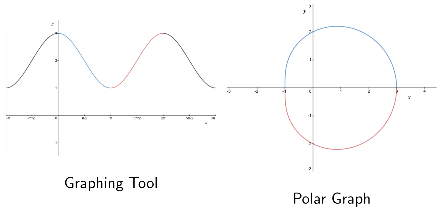
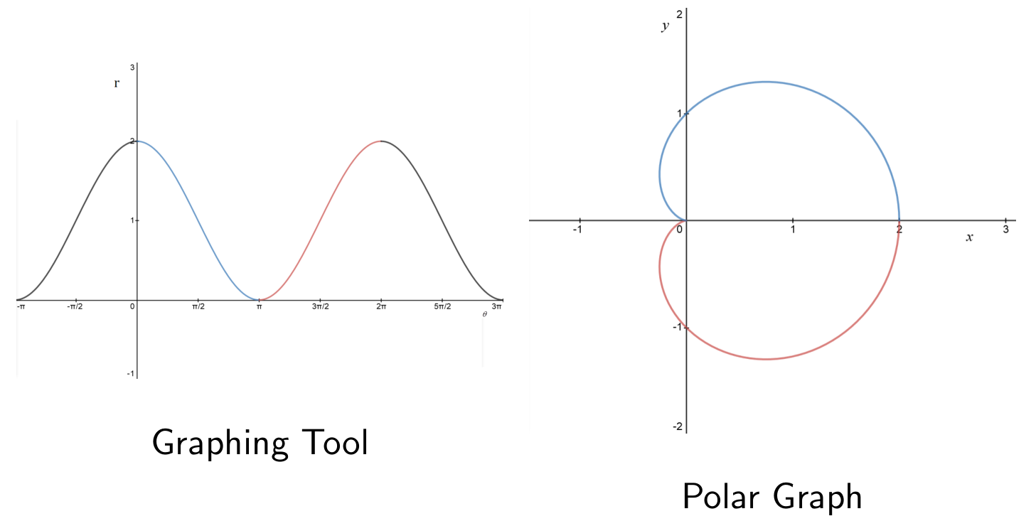
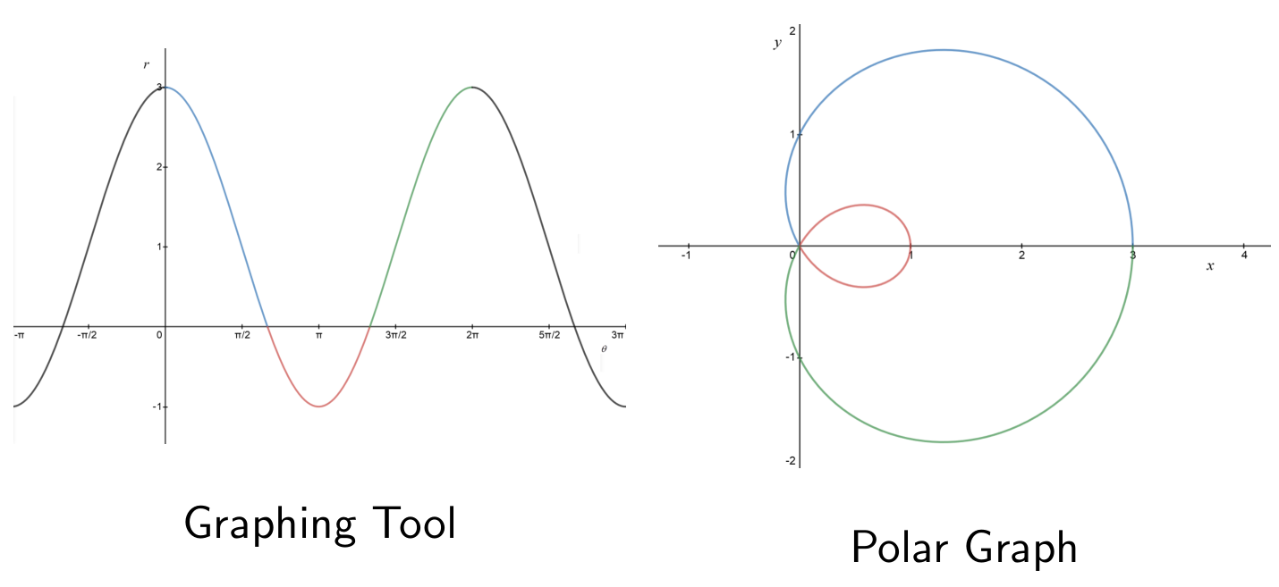
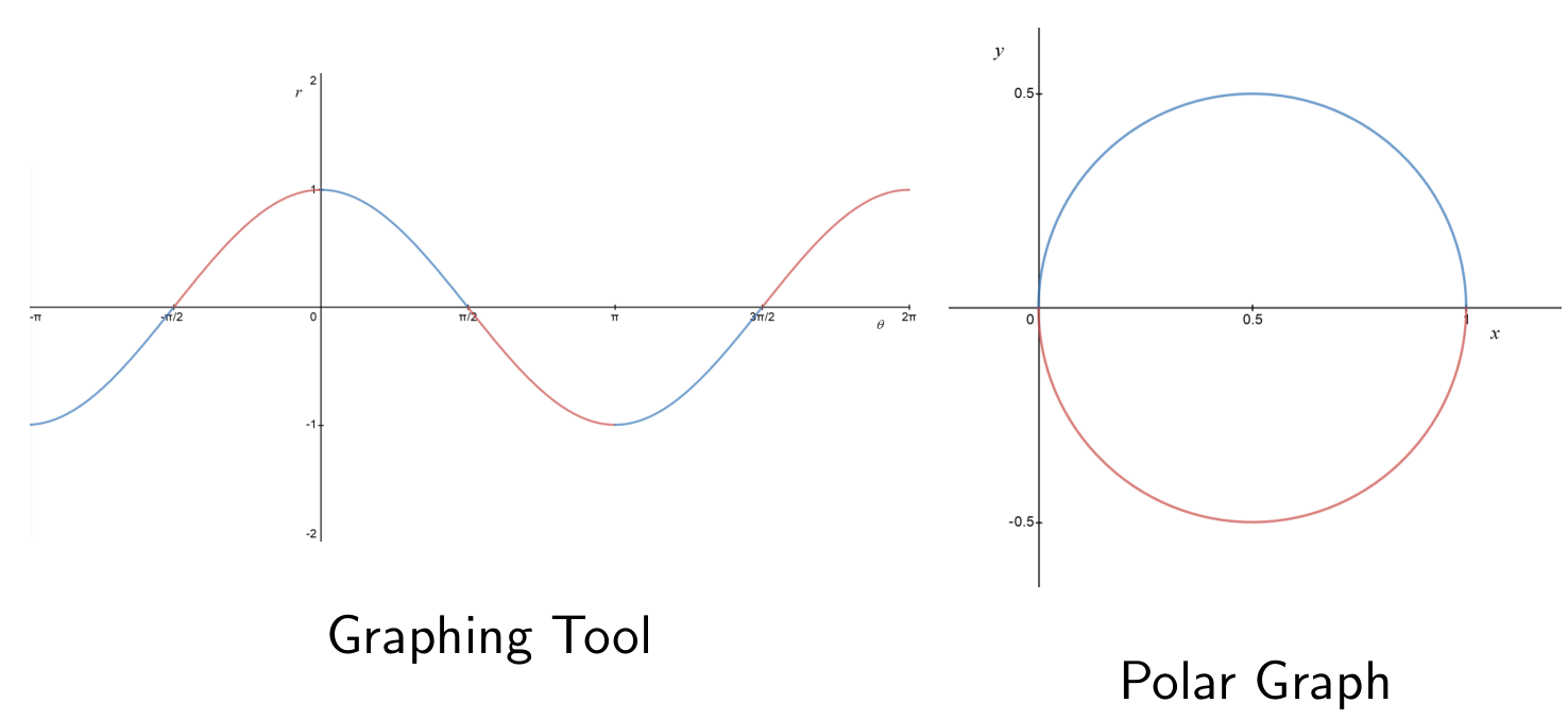
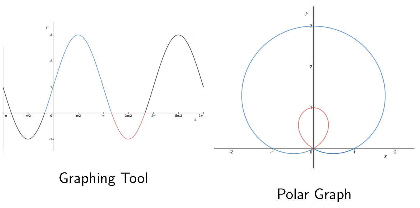
To draw the polar graph of some function, it can help to first draw the Cartesian graph of the function. (In other words, set $y=r$ and $x=\theta$, and draw the usual graph.) By tracing through the points on the Cartesian graph, one can visualize the trajectory of the polar graph.

This Cartesian graph may be called a graphing tool for the polar graph.

---

A limaçon is the polar graph of $r(\theta )=a+b\cos \theta$.

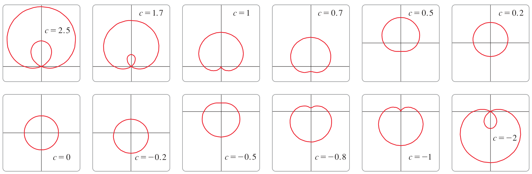
The shape of a limaçon is determined by the value of $c=\frac{b}{a}$. Any limaçon can be rescaled to have this form:

$$r=1+c\cos \theta$$

$c=0$: Limaçon satisfying $r(\theta )=1$: unit circle.

$c=0.5$: Limaçon satisfying $r(\theta )=2+\cos \theta$: ‘outer loop’ circle with ‘flat spot’, not quite a ‘dimple’:

$c=1$: Limaçon satisfying $r(\theta )=1+\cos \theta$: ‘cardioid’ $=$ ‘outer loop’ circle with ‘dimple’ that creates a cusp:

$c=2$: Limaçon satisfying $r(\theta )=1+2\cos \theta$: ‘dimple’ pushes past cusp to create ‘inner loop’:

$c=\infty$: Limaçon satisfying $r(\theta )=\cos \theta$: ‘inner loop’ only, no outer loop exists:

$c=2$: Limaçon satisfying $r(\theta )=1+2\sin \theta$: ‘inner loop’ and ‘outer loop’ and rotated $\circlearrowleft 90^{\circ }$:

---

Transitions between limaçon types, $r(\theta )=1+c\sin \theta$:

Notice the transition points at $|c|=0.5$ and $|c|=1$:

The flat spot occurs when $c=\pm 0.5$

• Smaller $c$ gives convex shape

The cusp occurs when $c=\pm 1$

• Smaller $c$ gives dimple (assuming $|c|>0.5$)
• Larger $c$ gives inner loop

Link to original

Theory - Polar roses

Theory 3

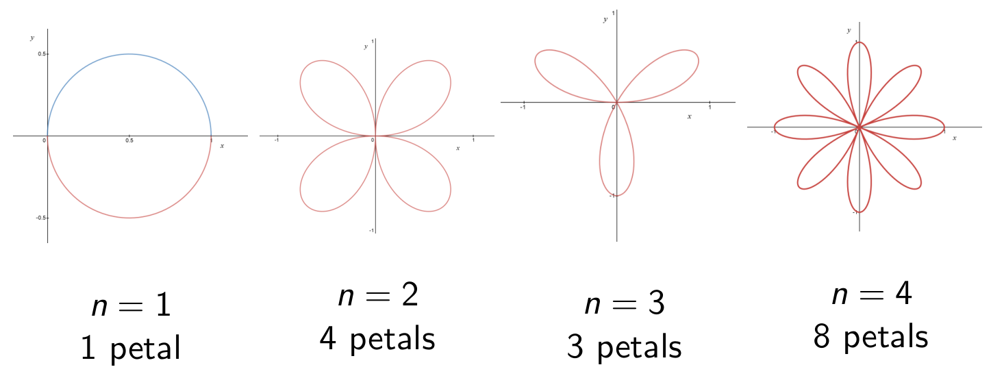
Roses are polar graphs of this form:

$$r=\cos (\theta ),r=\sin (2\theta ),r=\sin (3\theta ),r=\cos (4\theta )$$

The pattern of petals:

• $n=2k$ (even): obtain $2n$ petals
  • These petals traversed once
• $n=2k+1$ (odd): obtain $n$ petals
  • These petals traversed twice
• Either way: total-petal-traversals: always $2n$

Link to original

Illustration

Example - Finding vertical tangents to a limaçon

Finding vertical tangents to a limaçon

Let us find the vertical tangents to the limaçon (the cardioid) given by $r=1+\sin \theta$.

Solution

(1) Convert to Cartesian parametric using $x=r\cos \theta$ and $y=r\sin \theta$:

$$r(\theta )=1+\sin \theta \gg \gg (x,y)=((1+\sin \theta )\cos \theta ,(1+\sin \theta )\sin \theta )$$

---

(2) Compute $x^{\prime }$ and $y^{\prime }$:

$$\begin{array}{c}(x^{\prime }(\theta ),y^{\prime }(\theta ))\\ \\ \gg \gg (\cos \theta \cos \theta +(1+\sin \theta )(-\sin \theta ),\cos \theta \sin \theta +(1+\sin \theta )\cos \theta )\\ \\ \gg \gg ({\cos }^2\theta -{\sin }^2\theta -\sin \theta ,\cos \theta (1+2\sin \theta ))\end{array}$$

---

(3) The vertical tangents occur when $x^{\prime }(\theta )=0$. We must double check that $y^{\prime }(\theta )\ne 0$ at these points.

$$\begin{array}{c}{x}^{\prime }(\theta )=0\gg \gg {\cos }^2\theta -{\sin }^2\theta -\sin \theta =0\\ \\ \gg \gg (1-{\sin }^2\theta )-{\sin }^2\theta -\sin \theta =0\end{array}$$

Substitute $A=\sin \theta$ and observe quadratic:

$$\gg \gg 1-2A^2-A=0\gg \gg 2A^2+A-1=0$$

Solve:

$$\begin{array}{c}A=\frac{-b\pm \sqrt{b^2-4ac}}{2a}\gg \gg \\ \\ \frac{-1\pm \sqrt{1-4\cdot 2\cdot (-1)}}{2\cdot 2}\gg \gg \frac{1}{2},-1\end{array}$$

Then find $\theta$:

$$\begin{array}{c}A=\sin \theta \gg \gg \sin \theta =\frac{1}{2},-1\\ \\ \gg \gg \theta =\frac{\pi }{6},\frac{5\pi }{6}(\text{for }1/2)\text{and}\theta =\frac{3\pi }{2}(\text{for }-1)\end{array}$$

---

(4) Compute the points. In polar coordinates:

$$\begin{array}{c}(r,\theta )=(1+\sin \theta ,\theta ){|}_{\theta =\frac{\pi }{6},\frac{5\pi }{6},\frac{3\pi }{2}}\\ \\ \gg \gg \left(\frac{3}{2},\frac{\pi }{6}\right),\left(\frac{3}{2},\frac{5\pi }{6}\right),\left(0,\frac{3\pi }{2}\right)\end{array}$$

In Cartesian coordinates:

At $\theta =\frac{\pi }{6}$:

$$\begin{array}{c}(x,y){|}_{\theta =\frac{\pi }{6}}\gg \gg ((1+\sin \theta )\cos \theta ,(1+\sin \theta )\sin \theta ){|}_{\theta =\frac{\pi }{6}}\\ \\ \gg \gg \left(\left(1+\frac{1}{2}\right)\frac{\sqrt{3}}{2},\left(1+\frac{1}{2}\right)\frac{1}{2}\right)\gg \gg \left(\frac{3\sqrt{3}}{4},\frac{3}{4}\right)\end{array}$$

At $\theta =\frac{5\pi }{6}$:

$$\begin{array}{c}(x,y){|}_{\theta =\frac{5\pi }{6}}\gg \gg ((1+\sin \theta )\cos \theta ,(1+\sin \theta )\sin \theta ){|}_{\theta =\frac{5\pi }{6}}\\ \\ \gg \gg \left(\left(1+\frac{1}{2}\right)\frac{-\sqrt{3}}{2},\left(1+\frac{1}{2}\right)\frac{1}{2}\right)\gg \gg \left(-\frac{3\sqrt{3}}{4},\frac{3}{4}\right)\end{array}$$

At $\theta =\frac{3\pi }{2}$:

$$\begin{array}{c}(x,y){|}_{\theta =\frac{3\pi }{2}}\gg \gg ((1+\sin \theta )\cos \theta ,(1+\sin \theta )\sin \theta ){|}_{\theta =\frac{3\pi }{2}}\\ \\ \gg \gg ((1-1)\cdot 0,(1-1)\cdot (-1))\gg \gg (0,0)\end{array}$$

---

(5) Correction: $(0,0)$ is a cusp!

The point $(0,0)$ at $\theta =\frac{3\pi }{2}$ is on the cardioid, but the curve is not smooth there, this is a cusp.

Still, the left- and right-sided tangents exists and are equal, so in a certain sense we could say the curve has vertical tangent at $\theta =\frac{3\pi }{2}$.

Link to original

Calculus with polar curves

Theory - Polar tangent lines, arclength

Theory 1

Polar arclength formula

The arclength of the polar graph of $r(\theta )$, for $\theta \in [\alpha ,\beta ]$:

$$L={\int }_{\alpha }^{\beta }\sqrt{r^{\prime }(\theta {)}^2+r(\theta {)}^2}d\theta$$

To derive this formula, convert to Cartesian with parameter $\theta$:

$$r=r(\theta )\gg \gg (x,y)=(r\cos \theta ,r\sin \theta )$$

From here you can apply the familiar arclength formula with $\theta$ in the place of $t$.

Extra - Derivation of polar arclength formula

Let $r=r(\theta )$ and convert to parametric Cartesian, so:

$$\begin{array}{rl}x(\theta )& =r(\theta )\cos \theta \\ y(\theta )& =r(\theta )\sin \theta \end{array}$$

Then:

$$\begin{array}{c}ds=\sqrt{(x^{\prime }{)}^2+(y^{\prime }{)}^2}d\theta \\ \\ x^{\prime }=(r\cos \theta {)}^{\prime }\gg \gg r^{\prime }\cos \theta -r\sin \theta \\ y^{\prime }=(r\sin \theta {)}^{\prime }\gg \gg r^{\prime }\sin \theta +r\cos \theta \end{array}$$

Therefore:

$$\begin{array}{rl}(x^{\prime }{)}^2+(y^{\prime }{)}^2\gg \gg & r^{\prime 2}{\cos }^2\theta -2r{r}^{\prime }\cos \theta \sin \theta +r^2{\sin }^2\theta \\ & +r^{\prime 2}{\sin }^2\theta +2r{r}^{\prime }\sin \theta \cos \theta +r^2{\cos }^2\theta \\ & \\ & =r^{\prime 2}+r^2\end{array}$$

Therefore:

$$ds=\sqrt{(x^{\prime }{)}^2+(y^{\prime }{)}^2}d\theta \gg \gg \sqrt{r^{\prime 2}+r^2}d\theta$$

Link to original

Illustration

Example - Length of the inner loop

Length of the inner loop

Consider the limaçon given by $r(\theta )=\frac{1}{2}+\cos \theta$.

How long is the inner loop? Set up an integral for this quantity.

Solution

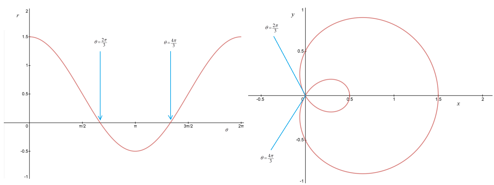
The inner loop is traced by the moving point when $\frac{2\pi }{3}\le \theta \le \frac{4\pi }{3}$. This can be seen from the graph:

Therefore the length of the inner loop is given by this integral:

$$L={\int }_{2\pi /3}^{4\pi /3}\sqrt{(-\sin \theta {)}^2+{\left(\frac{1}{2}+\cos \theta \right)}^2}d\theta \gg \gg {\int }_{2\pi /3}^{4\pi /3}\sqrt{5/4+\cos \theta }d\theta$$ Link to original

Theory - Polar area

Theory 2

Sectorial area from polar curve

$$A={\int }_{\alpha }^{\beta }\frac{1}{2}r(\theta {)}^{2}d\theta$$

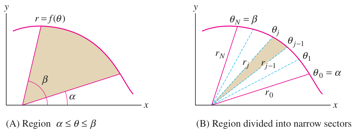
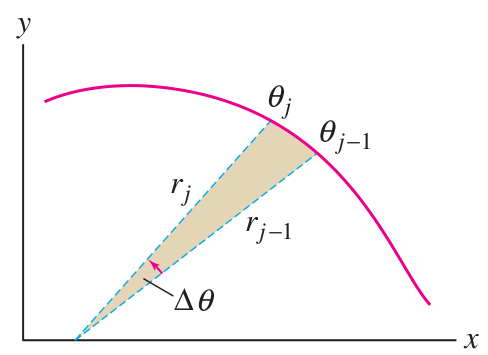
The “area under the curve” concept for graphs of functions in Cartesian coordinates translates to a “sectorial area” concept for polar graphs. To compute this area using an integral, we divide the region into Riemann sums of small sector slices.

To obtain a formula for the whole area, we need a formula for the area of each sector slice.

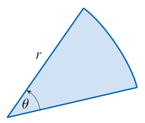
Area of sector slice

Let us verify that the area of a sector slice is $\frac{1}{2}{r}^2\theta$.

Take the angle $\theta$ in radians and divide by $2\pi$ to get the fraction of the whole disk.

Then multiply this fraction by $\pi r^2$ (whole disk area) to get the area of the sector slice.

$$\left(\frac{\theta }{2\pi }\right)\left(\pi r^2\right)\gg \gg \frac{1}{2}{r}^2\theta$$

Now use $d\theta$ and $r(\theta )$ for an infinitesimal sector slice, and integrate these to get the total area formula:

$$A={\int }_{\alpha }^{\beta }\frac{1}{2}r(\theta {)}^{2}d\theta$$

---

One easily verifies this formula for a circle.

Let $r(\theta )=R$ be a constant. Then:

$$\text{Area of circle}={\int }_0^{2\pi }\frac{1}{2}{R}^{2}d\theta \gg \gg \frac{1}{2}{R}^2\theta {|}_0^{2\pi }\gg \gg R^2\pi$$

---

The sectorial area between curves:

Sectorial area between polar curves

$$A={\int }_{\alpha }^{\beta }\frac{1}{2}(r_1(\theta {)}^2-r_0(\theta {)}^2)d\theta$$

Subtract after squaring, not before!

This aspect is not similar to the Cartesian version: $\int f-gdx$

Link to original

Illustration

Area between circle and limaçon

Area between circle and limaçon

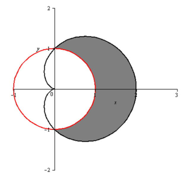
Find the area of the region enclosed between the circle $r_0(\theta )=1$ and the limaçon $r_1(\theta )=1+\cos \theta$.

Solution

First draw the region:

The two curves intersect at $\theta =\pm \frac{\pi }{2}$. Therefore the area enclosed is given by integrating over $-\frac{\pi }{2}\le \theta \le +\frac{\pi }{2}$:

$$\begin{array}{c}A={\int }_{\alpha }^{\beta }\frac{1}{2}(r_1^2-r_0^2)d\theta \gg \gg {\int }_{-\pi /2}^{\pi /2}\frac{1}{2}((1+\cos \theta {)}^2-1^2)d\theta \\ \\ \gg \gg \frac{1}{2}{\int }_{-\pi /2}^{\pi /2}2\cos \theta +{\cos }^2\theta d\theta \gg \gg {\int }_{-\pi /2}^{\pi /2}\cos \theta +\frac{1}{4}(1+\cos (2\theta ))d\theta \\ \\ \gg \gg {\sin \theta +\frac{\theta }{4}+\frac{1}{8}\sin (2\theta )|}_{-\pi /2}^{\pi /2}\gg \gg 2+\frac{\pi }{4}\end{array}$$ Link to original

Area of small loops

Area of small loops

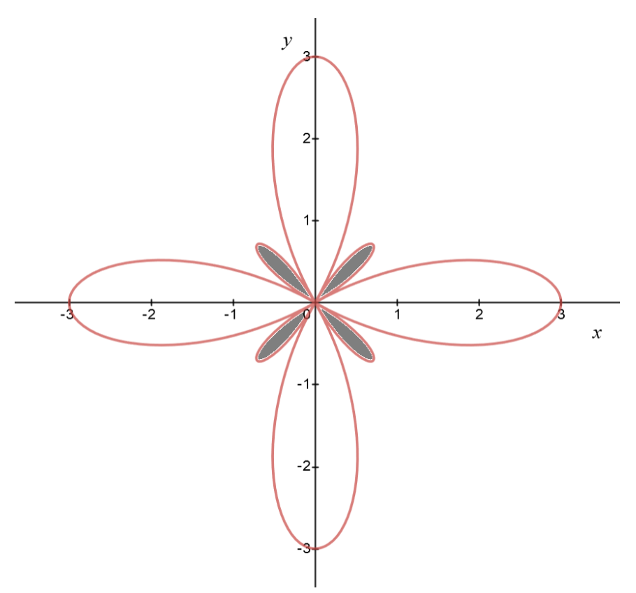
Consider the following polar graph of $r(\theta )=1+2\cos (4\theta )$:

Find the area of the shaded region.

Solution

Find bounds for one small loop. Lower left loop occurs first. This loop is when $1+2\cos (4\theta )\le 0$.

$$\begin{array}{c}1+2\cos (4\theta )\le 0\gg \gg \cos (4\theta )\le -\frac{1}{2}\\ \\ \gg \gg \frac{2\pi }{3}\le 4\theta \le \frac{4\pi }{3}\gg \gg \frac{\pi }{6}\le \theta \le \frac{\pi }{3}\end{array}$$

Now set up area integral:

$$\begin{array}{c}A=4{\int }_{\alpha }^{\beta }\frac{1}{2}r(\theta {)}^{2}d\theta \gg \gg 4{\int }_{\pi /6}^{\pi /3}\frac{1}{2}(1+2\cos (4\theta ){)}^{2}d\theta \\ \\ \gg \gg 2{\int }_{\pi /6}^{\pi /3}1+4\cos (4\theta )+4{\cos }^2(4\theta )d\theta \end{array}$$

Power-to-frequency conversion: ${\cos }^{2}A⇝\frac{1}{2}(1+\cos (2A))$ with $A=4\theta$:

$$\begin{array}{c}\gg \gg 2{\int }_{\pi /6}^{\pi /3}1+4\cos (4\theta )+4\cdot \frac{1}{2}(1+\cos (8\theta ))d\theta \\ \\ \gg \gg {6\theta +2\sin (4\theta )+\frac{1}{4}\sin (8\theta )|}_{\pi /6}^{\pi /3}\gg \gg \pi -\frac{3\sqrt{3}}{2}\end{array}$$ Link to original

Overlap area of circles

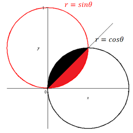
Overlap area of circles

Compute the area of the overlap between crossing circles. For concreteness, suppose one of the circles is given by $r(\theta )=\sin \theta$ and the other is given by $r(\theta )=\cos \theta$.

Solution

Drawing of the overlap:

Notice: total overlap area = $2\times$ area of red region. Bounds for red region: $0\le \theta \le \frac{\pi }{4}$.

Area formula applied to $r(\theta )=\sin \theta$:

$$A=2{\int }_{\alpha }^{\beta }\frac{1}{2}r(\theta {)}^{2}d\theta \gg \gg 2{\int }_0^{\pi /4}\frac{1}{2}{\sin }^2\theta d\theta$$

Power-to-frequency: ${\sin }^2\theta ⇝\frac{1}{2}(1-\cos (2\theta ))$:

$$\begin{array}{c}\gg \gg 2{\int }_0^{\pi /4}\frac{1}{4}(1-\cos (2\theta ))d\theta \\ \\ \gg \gg \frac{2}{4}\theta -{\frac{2}{8}\sin (2\theta )|}_0^{\pi /4}\gg \gg \frac{\pi }{8}-\frac{1}{4}\end{array}$$Link to original