Theory

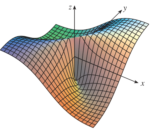
Introduction

Suppose we are given a function $f:{\mathbb{R}}^2\to \mathbb{R}$, written in terms of components by $f(x,y)\in \mathbb{R}$ for each $(x,y)\in {\mathbb{R}}^2$. Now let the second coordinate remain some arbitrary fixed value $y=b$. This determines a function $f(x,b)$ of one variable, $x$, for each possible chosen $b$.

We can take the derivative of $f(x,y_0)$ in $x$ just as any other function of $x$:

$$\frac{d}{dx}f(x,b)=\underset{h\to 0}{\lim }\frac{f(x+h,b)-f(x,b)}{h}.$$

The resulting function of $x$ may be considered for various possible values of $b$, i.e. the variation may be restored. This function of both $x$ and $y$ is called the partial derivative of $f$ with respect to $x$. As with ordinary derivatives, a variety of notations is used:

$$f_x(x,y)=\frac{\partial }{\partial x}f(x,y)=\frac{\partial f}{\partial x}(x,y)=\underset{h\to 0}{\lim }\frac{f(x+h,y)-f(x,y)}{h}.$$

The new symbol ‘ $\partial$ ’ is called “partial” and should be written differently from ‘ $d$ ’. This symbol indicates the function’s dependence on additional variables.

Functions of several variables may have partial derivatives in each of their variables. Thus, for $f$ above we also have $f_y$ or $\frac{\partial f}{\partial y}$.

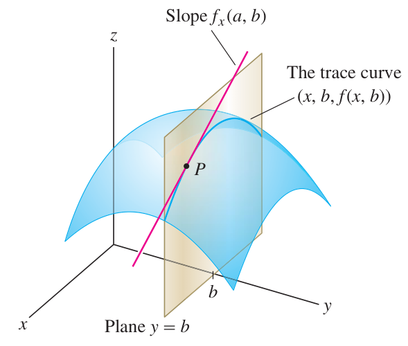
By interpreting the function $f(x,b)$ as the “trace” of the function $f(x,y)$ at a fixed value $y=b$, one sees that the partial derivative gives the slope of the curve formed as the cross-section of the plane $y=b$ with the graph of $f$, namely the surface $z=f(x,y)$:

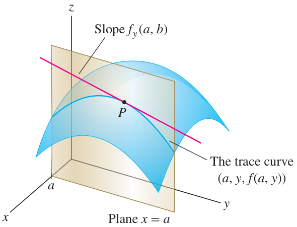
Similarly for the partial $f_y$ and the trace $x=a$:

One can iterate partial derivatives and consider higher partials in the obvious manner. The notation $f_{xy}$ indicates the “mixed partial” taken in $x$ first:

$$f_{xy}=\frac{\partial }{\partial y}\left(\frac{\partial f}{\partial x}\right)=\frac{{\partial }^{2}f}{\partial y\partial x}.$$

In principle, the double partials $f_{xy}$ and $f_{yx}$ could be different, but for nice functions they do agree by Clairaut’s Theorem:

Clairaut’s Theorem

Provided $f_{xy}$ and $f_{yx}$ exist and are continuous on a region $\mathcal{R}$, then $f_{xy}=f_{yx}$ on that region.

(Caveat: in the theorem, $\mathcal{R}$ should be ‘open’ topologically: it should have the same dimension as the background and not include its boundary.)

Introduction (part 2)

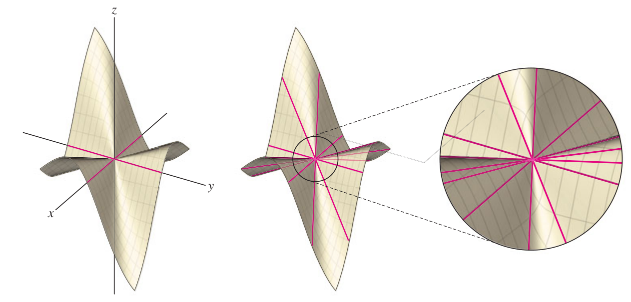
Continuity and differentiability: more complex in 3d!

The concepts of continuity and differentiability are more complicated in 3d due to potential incompatibilities of directionality that are a function of the $x$ and $y$ relationship.
$z=f(x,y)=\frac{xy}{x^2+y^2}$

$z=f(x,y)=\frac{2xy(x+y)}{x^2+y^2}$