Theory

Introduction

A real-valued function $f(x,y)$ may be called a scalar field. The word ‘field’ indicates a mathematical structure that assigns a concrete object of a certain fixed type to every point in space. A function $f$ may be interpreted as assigning a scalar value, the output $f(x,y)$, to each point in space.

A vector field $\mathbf{F}$ assigns a vector value to each point of space. The data of a vector field can be conveyed as a collection of coordinate functions, where each coordinate function takes a point $p$ in space as input:

$$\mathbf{F}(x,y)=(F_1(x,y),F_2(x,y)).$$

(In 3D, the vector field has 3 coordinate functions.) We can also represent the same data as:

$$\mathbf{F}(p)=F_1(p){\mathbf{e}}_{\mathbf{i}}+F_2(p){\mathbf{e}}_{\mathbf{j}}.$$

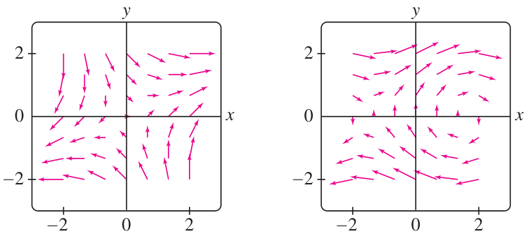
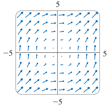
Vector fields in 3D are harder to visualize:

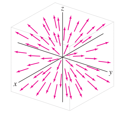
Vector fields are often used to represent a fluid flow (the vector gives flow velocity) or a force field (vector gives force). Both types of data require the assignment of a vector to each point in space.

Gradient

Given a function $f(x,y)$, a natural vector field may be formed using its partial derivative functions. This is called the gradient of $f$, and $f$ is called the potential function of this vector field:

$$\nabla f=\left(\frac{\partial f}{\partial x},\frac{\partial f}{\partial y}\right)=(f_x,f_y).$$

In 3D, the gradient of $f(x,y,z)$ has components $\nabla f=(f_x,f_y,f_z)$.

Recall that the partial $f_x$ is large when $f$ increases steeply in the $+x$ direction, and it is large and negative when $f_x$ increases steeply in the $-x$ direction. These facts generalize with the combined components: $\nabla f$ points in the direction of steepest increase of $f$. This can be understood by recalculating the formula for $D_{\mathbf{u}}(f)$:

Gradient and directional derivative

$$D_{\mathbf{u}}(f)=f_x\cdot h+f_y\cdot k=\nabla f\cdot \mathbf{u}$$

If we consider unit vectors $\mathbf{u}$ pointing in various directions, we see that the greatest value of $D_{\mathbf{u}}(f)$ occurs when $\mathbf{u}$ aligns with $\nabla f$. This means that $\nabla f$ points in the direction in which $D_{\mathbf{u}}(f)$ is largest, i.e. the direction of steepest incline.

Gradient (part 2)

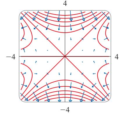
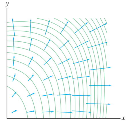
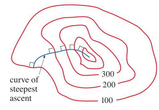
The level curves of a function $f(x,y)$ are the sets of points satisfying $f(x,y)=c$ for various $c\in \mathbb{R}$. The gradient vector is perpendicular to the level curves:

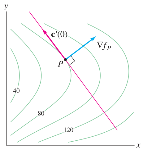
Proposition: Gradient $\perp$ level curves

The level curves to $f$ are perpendicular to the gradient vector.

Proof: Let $\mathbf{r}(t)$ parametrize the level curve $f(x,y)=c$, so $f(\mathbf{r}(t))=c$ for all $t$. Then:

$$0=\frac{d}{dt}c=\frac{d}{dt}f(\mathbf{r}(t))=\nabla f\cdot {\mathbf{r}}^{\prime }(t),$$

so $\nabla f\perp {\mathbf{r}}^{\prime }(t)$.

This result can be generalized to surfaces. The level surfaces of a function $f$ are given by $f(x,y,z)=k$. Any curve $\mathbf{r}(t)$ in such a level surface satisfies $f(\mathbf{r}(t))=k$, and therefore $0=\frac{d}{dt}f(\mathbf{r}(t))=\nabla f\cdot {\mathbf{r}}^{\prime }(t)$. This means the tangent plane to a level surface $f(x,y,z)=k$ has normal vector given by $\mathbf{n}=\nabla f$ at any given point.

Gradient (part 3)

If you follow the gradient vectors, you will go up or down a path of steepest ascent. This is also the path that crosses levels curves most quickly.