Theory

Review of 1D theory

A regular point of a function $f$ is a point $c$ where $f^{\prime }(c)=m\ne 0$. A critical point is a point $c\in \mathbb{R}$ where $f^{\prime }(c)$ is either zero or undefined. In calculus, the theory of optimization (finding extremal values) is largely a theory of critical points.

Given a function $f(x)$ of a single variable, its extrema occur either on boundary points of the region, or at critical points of $f$ in the interior of the region. For a closed interval $[a,b]$, the boundary points are $a$ and $b$, while the interior is the open interval $(a,b)$. Every interior point is either regular or critical. To find extrema, therefore, it suffices to check boundary points, interior points of non-differentiability, and interior points where the derivative is zero.

All of this reasoning may be derived from the linear approximation:

Linear approximation: $f^{\prime }(c)\ne 0⟹\text{local increase/decrease possible}$

If $f^{\prime }(x)$ exists at $c$, we can write $f$ near $c$ as:

$$f(x)=b+m\Delta x+\Delta x\epsilon (\Delta x).$$

Here $f(c)=b$, $f^{\prime }(c)=m$, and $\Delta x=x-c$. Now rewrite this as $f(x)=b+(m+\epsilon )\Delta x$. If $m>0$, then for $\Delta x$ small enough, $m+\epsilon >0$ because $\epsilon \to 0$ as $\Delta x\to 0$. This means there are points $a$ close to $c$ for which $f(a)>f(c)$ (with $a>c$), and points for which $f(a)<f(c)$ (with $a<c$). Conversely, if $m<0$, there are points $a$ near $c$ for which $f(a)<f(c)$ and for which $f(a)>f(c)$.

It follows that if $c$ is a regular point, meaning $f^{\prime }(c)=m\ne 0$, then $c$ is certainly neither a local maximum nor minimum.

The critical points can be evaluated using the first and second derivative tests. For example, if the sign of $f^{\prime }$ crosses zero at $c$ from above, or if $f^{\prime \prime }(c)<0$, the point is a local maximum.

2D theory

The 1D theory may be applied directly to the trace curves of a function $f(x,y)$, i.e. the curves given by $z=f(x,b)$ or $z=f(a,y)$. The result is that if $f_x(a,b)=m_x\ne 0$, or if $f_y(a,b)=m_y\ne 0$, then $(a,b)$ is neither a local maximum nor minimum, but rather it would be possible to increase or decrease $f$ by moving along the respective trace curve.

A critical point of $f(x,y)$ is a point $(a,b)$ such that either $f_x(a,b)=f_y(a,b)=0$, or at least one of $f_x,f_y$ doesn’t exist. All extreme values of $f(x,y)$ in the interior of a region must occur, therefore, at critical points.

(Note: the situation where, say, $f_y$ fails to exist while $f_x=m_x\ne 0$, counts as a critical point in these notes, but some other authors would not count it. Such points cannot be local extrema by the trace-curve reasoning applied to $x$.)

The definition of critical points can be encapsulated in a single statement about the gradient:

Info

The point $p$ is a critical point of $f$ if and only if: $\nabla f(p)=\vec{0}$ or $\nabla f(p)$ is undefined.

Global extrema are either local extrema (critical points in the interior), or they lie on the boundary. To check the boundary, one must find a parametrization of the boundary as a curve $\mathbf{r}(t)$, and then optimize the scalar function $f(\mathbf{r}(t))$ of the single variable $t$ using the 1D theory. The extrema on the boundary should then be compared with the local extrema in the interior.

As in the 1D theory, critical points of $f(x,y)$ can be either maxima or minima or neither, and there is a tool involving second-order partials that allows us to classify critical points in many cases. It is called the discriminant. Suppose that $f_{xx},f_{yy},f_{xy}$ exist and are continuous near $(a,b)$, a critical point of $f(x,y)$. Define the discriminant $D(x,y)$ by the formula:

$$D(x,y)=f_{xx}(x,y)f_{yy}(x,y)-f_{xy}(x,y{)}^2.$$

This formula is easy to remember as the determinant of the matrix of second-order partials:

$$D=\left|\begin{array}{cc}{f}_{xx}& f_{xy}\\ f_{yx}& f_{yy}\end{array}\right|.$$

Discriminant test

Let $(a,b)$ be a critical point near which the second-order partials are continuous.

• If $D(a,b)=0$ the test is inconclusive
• If $D(a,b)<0$ then $(a,b)$ is a saddle point
• If $D(a,b)>0$ then $(a,b)$ is a max/min:
  • If $f_{xx}>0$ or $f_{yy}>0$ then $(a,b)$ is a min
  • If $f_{xx}<0$ or $f_{yy}<0$ then $(a,b)$ is a max

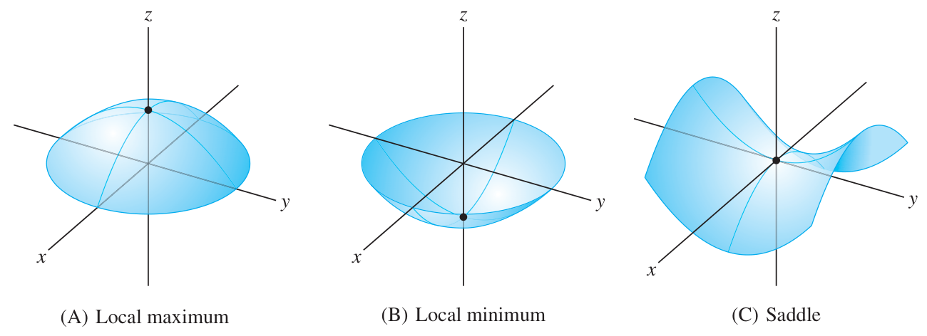
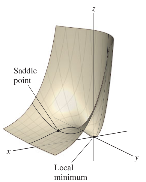
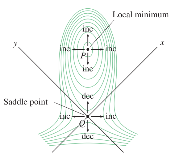
nD theory

(The technique for $n$D requires knowledge of linear algebra, so the next discussion will not be tested in this course.)

In 3D, the same argument about trace curves shows that where $\nabla f=(f_x,f_y,f_z)$ is a non-zero vector, there $f$ is not a local extremum. At such a point, motion in the direction of $\nabla f$ will increase the value of $f$, and motion in the (opposite) direction of $-\nabla f$ will decrease the value of $f$.

Similarly, in $n$D one defines critical points as those points $p$ where $\nabla f(p)$ is either $\vec{0}$ or undefined. Local extrema of $f(x_1,\dots ,x_n)$ can only occur at critical points.

The matrix of second-order partials has a general form called the Hessian matrix:

$$H(x_1,\dots ,x_n)=\left(\begin{array}{ccc}{f}_{x_1{x}_1}& \dots & f_{x_1{x}_n}\\ \dots & \dots & \dots \\ f_{x_n{x}_1}& \dots & f_{x_n{x}_n}\end{array}\right).$$

In 3D the Hessian matrix looks like this:

$$H(x,y,z)=\left(\begin{array}{ccc}{f}_{xx}& f_{xy}& f_{xz}\\ f_{yx}& f_{yy}& f_{yz}\\ f_{zx}& f_{zy}& f_{zz}\end{array}\right).$$

In order to use $H(x,y,z)$ to classify critical points, you have to compute its eigenvalues and count the number of positive and number of negative eigenvalues. (All positive $⇝$ minimum, all negative $⇝$ maximum, various signs $⇝$ saddle.) The determinant is the product of the eigenvalues, so in the 2D theory the discriminant reveals whether the eigenvalues have the same or opposite signs. This explains the discriminant rule that is used in 2D.