Theory

Introduction

The setup is a function $f(x,y)$ and a curve $\mathcal{C}$. The problem is to find the extremal values of $f(x,y)$ on the curve. If the curve $\mathcal{C}$ is given with a parametrization $\mathbf{r}(t)$, then we could just extremize $f(\mathbf{r}(t))$ using the 1D theory. If the curve is instead given by a constraint such as $g(x,y)=0$, then there is another technique that can be much easier to implement than finding a parametrization $\mathbf{r}(t)$ for $\mathcal{C}$. It is called Lagrange multipliers. Since the constraint is written as $g(x,y)=0$, you can think of this as a relative of implicit differentiation.

The method of Lagrange multipliers makes use of the fact that when $f(x,y)$ is extremized at $p$ on $g(x,y)=0$, then the gradients must align: $\nabla f(p)=\lambda \nabla g(p)$ for some scalar $\lambda$.

Gradients align at extremal values

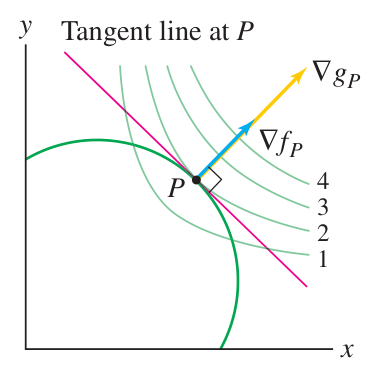
The constraint curve $\mathcal{C}$ is given as the level curve $g(x,y)=c$ with $c=0$. To show the gradients align, we show that they are both perpendicular to this level curve.
Let $\mathbf{r}(t)$ be a parametrization of $\mathcal{C}$. We have already seen that:

$$0=\frac{d}{dt}0=\frac{d}{dt}g(\mathbf{r}(t))=\nabla g\cdot {\mathbf{r}}^{\prime }(t)$$

for any $t$, so $\nabla g$ is always perpendicular to the level curves. In addition, at the specific time $t_0$ where $f(\mathbf{r}(t))$ is extremized, we also have from the 1D optimization theory and the chain rule:

$$0={\frac{d}{dt}f(\mathbf{r}(t))|}_{t_0}=\nabla f(\mathbf{r}(t_0))\cdot {\mathbf{r}}^{\prime }(t_0),$$

and this shows that $\nabla f$ is also perpendicular to the level curve $g(x,y)=0$ at $t_0$. Since both are perpendicular to the level curve, they must point along the same line.

Lagrange multipliers: parallel level curves

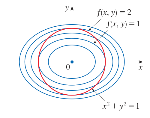
It is convenient to visualize the Lagrange condition on a contour map. The curve $\mathcal{C}$ will be parallel to the level curves of $f(x,y)$ at the points where the value of $f(x,y)$ is extremized on $\mathcal{C}$.

If the level curves of $f$ are not parallel to $\mathcal{C}$ at a point $p$, then it is possible to increase or decrease $f$ by moving along $\mathcal{C}$ because this motion will cross over level curves of $f$.

Because $\mathcal{C}$ is a level curve of $g(x,y)$, it is perpendicular to $\nabla g$. So the level curves of $g$ and $f$ must be parallel at an extremal point. This happens if and only if the gradients are parallel.