Theory

Introduction

The main theorem of 2D calculus is called Green’s Theorem, but it could be called more expressively “The Fundamental Theorem of 2D Calculus”. It says that the integral of curl over a region is equal to the total circulation on the boundary:

Green’s Theorem

When $\mathcal{D}$ is a region of the $xy$-plane with boundary $\partial \mathcal{D}$, then:

$${\iint }_{\mathcal{D}}\nabla {\times }_z\mathbf{F}dA={\oint }_{\partial \mathcal{D}}\mathbf{F}\cdot d\mathbf{s}$$

Writing this in terms of component functions, we have:

$${\iint }_{\mathcal{D}}\left(\frac{\partial F_2}{\partial x}-\frac{\partial F_1}{\partial y}\right)dxdy={\oint }_{\partial \mathcal{D}}{F}_{1}dx+F_{2}dy.$$

Understanding Green’s Theorem

To understand the reasoning behind Green’s Theorem, it is important to remember why the 1D version of the Fundamental Theorem of Calculus is true.

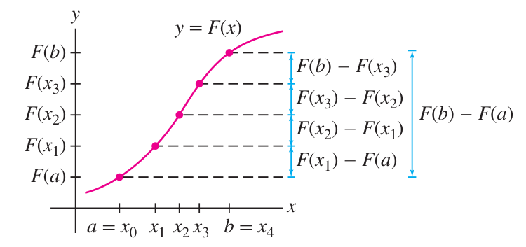
FTC derivation reminder: telescoping summation

Let $F^{\prime }(x)=f(x)$. We would like to see why ${\int }_a^{b}f(x)dx=F(b)-F(a)$.

If $a$ and $b$ are very close, we could write $F(b)=F(a)+f(a)\Delta x+\Delta x\epsilon (x)$. Ignoring the error term, we see that $F(b)-F(a)\approx f(a)\Delta x$, and the RHS is the area of a box with base $[a,b]$ and height $f(a)$. This is $\approx {\int }_a^{b}fdx$ when $\Delta x$ is very small.

If $a$ and $b$ are farther apart, divide $F(b)-F(a)$ into intervals:

$$\begin{array}{rl}F(b)-F(a)& =F(b)-F(x_{n-1})+F(x_{n-1})-F(x_{n-2})+\cdots +F(x_2)-F(a)\\ & =\sum _{i=1}^{n}F(x_{i+1})-F(x_i).\end{array}$$

Assume for simplicity that $x_{i+1}-x_i=\Delta x$ for every $i$. Now analyze each small difference using a linear approximation:

$$F(x_{i+1})=F(x_i)+f(x_i)\Delta x+\Delta x{\epsilon }_i(x).$$

Subtracting $F(x_i)$ from both sides and plugging into the summation, obtain:

$$F(b)-F(a)=\sum _{i=1}^{n}f(x_i)\Delta x+\sum _{i=1}^n\Delta x{\epsilon }_i(x).$$

If we ignore the error term and take the limit as $n\to \infty$ with $\Delta x\to 0$, then the first summation (a Riemann sum) becomes ${\int }_a^{b}fdx$.

To account for the error term properly, take $\Delta x$ small enough that $|{\epsilon }_i(x)|<\Delta xM$ for some fixed positive number $M$. Then as $n\to \infty$ the error summation limits to zero:

$$\left|\sum _{i=1}^n\Delta x{\epsilon }_i(x)\right|\le \sum _{i=1}^n\Delta x^{2}M=n\Delta x^{2}M=(b-a)\Delta xM\to 0.$$

To summarize, the key idea is that we add up all the small differences $F(x_{i+1})-F(x_i)$. In the sum, internal cancellation occurs, leaving just the boundary difference $F(b)-F(a)$. On the other hand, each small difference is approximated by $f(x_i)\Delta x$. (The linear approximation of $F$ using $F^{\prime }=f$.) The sum of these terms $f(x_i)\Delta x$ is exactly the Riemann sum for the integral ${\int }_a^{b}fdx$.

Even more briefly, the integral adds up many microscopic differences in $F$ which are written in the form $f(x_i)\Delta x$.

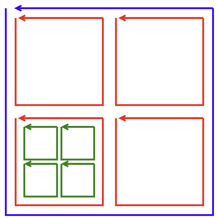
Green’s Theorem can be explained with exactly the same process, except that instead of differences, we have circulations, and instead of $f(x_i)\Delta x$ that approximates a small difference, we have $\nabla {\times }_z\mathbf{F}dA$ that approximates a small circulation. To add up circulations, we collect 2D squares, but there is still internal cancellation leaving only the terms on the boundary curve of the region.

Derivation of Green’s Theorem

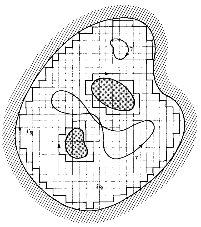
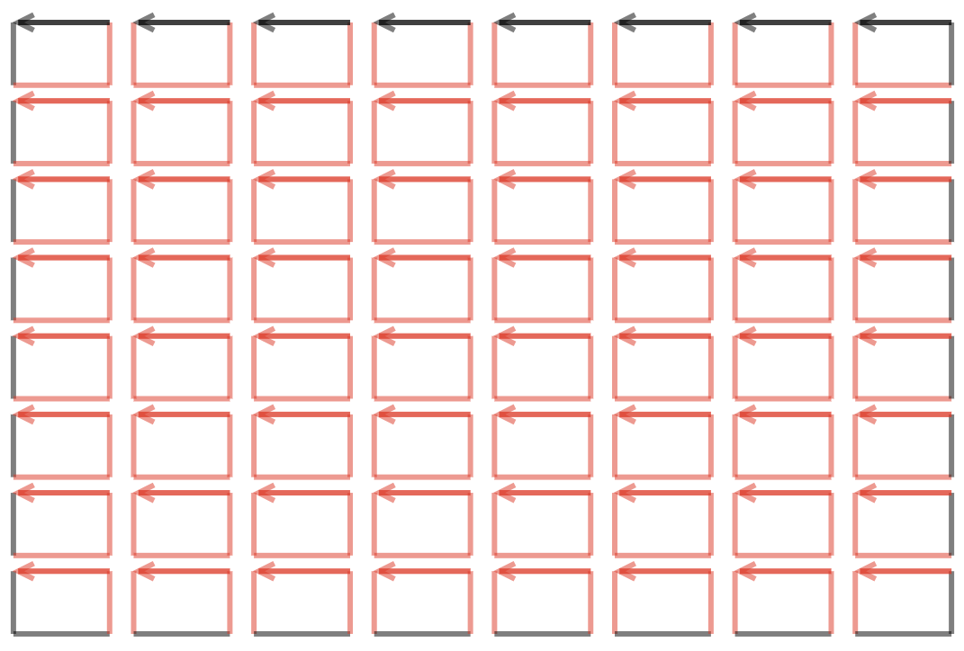
We need to divide the region $\mathcal{D}$ into microscopic squares. Let each square be identified by its bottom-left corner at point $(x_i,y_j)$, where $i,j\in 1,\dots ,n$. Each square has width and height $\Delta x=\Delta y=h$. Let ${\mathcal{I}}_n$ denote the set of squares fully contained inside $\mathcal{D}$ (specifically, the set of ordered pairs $(i,j)$ identifying the bottom-left corner of a square contained in $\mathcal{D}$).

The circulation around the square at $(x_i,y_j)$ is approximated by $h^2(\nabla {\times }_z\mathbf{F})(x_i,y_j)$. The error terms need to be collected as well; the exact circulation differs by an error term with magnitude less than $h^2\epsilon (h)$, where $\epsilon (h)$ is a positive function of $h$ satisfying $\epsilon (h)\le Mh$, for some $M$, as $h\to 0$. (Notice that this $\epsilon (h)$ can be chosen so it doesn’t depend on $(i,j)$ by taking the biggest one of those used for any of the squares in ${\mathcal{I}}_n$.)

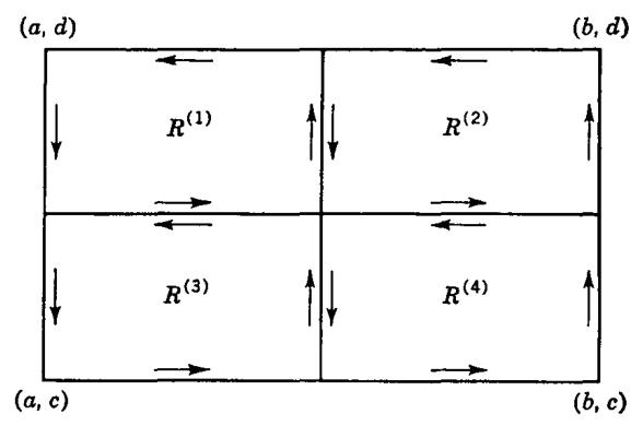
Now we add up all the circulations. The internal sides of boxes, which are shared between two boxes, will have a component of the integral traversed in each direction. These traversals contribute the same number with opposite signs, and therefore cancel. So, the total sum of circulations is equal to the circulation around the outer edges of the shape made by all squares of width $h$ which fit entirely in the domain. This is a 2D version of the cancellation in 1D that occurs between $F(x_{i+1})-F(x_i)$ and $F(x_i)-F(x_{i-1})$, for example.

Considering now the sum of approximations, we have the sum of the values $h^2(\nabla {\times }_z\mathbf{F})(x_i,y_j)$ multiplied by the area of the squares, $h^2$. This is a Riemann sum that limits to ${\int }_{\mathcal{D}}\nabla {\times }_z\mathbf{F}dA$ as $h\to 0$ and the number of boxes $n^2$ goes to $\infty$. So the circulations add up to the boundary circulation around the squares contained in $\mathcal{D}$, and the sum of approximations using $\nabla {\times }_z\mathbf{F}$ adds up to the integral of $\nabla {\times }_z\mathbf{F}$ over the region.

Now let’s address the error term. Each small square has an error less than $h^2\epsilon (h)$, which is less than $M{h}^3$ for some positive number $M$ based on the guarantees on the behavior of $\epsilon$. The number of boxes is $n^2$. Let’s say the total area of the region is $A$. The area covered by the boxes is $n^2{h}^2$ so $n^2{h}^2\le A$, and thus $n^2\le \frac{A}{h^2}$. The total error with all $n^2$ boxes is less than $M{h}^3{n}^2\le MhA$. But $MhA\to 0$ as $h\to 0$. So the total error goes to zero.

Going deeper

One remaining issue should be addressed. Does the boundary converge to the boundary $\partial \mathcal{D}=\mathcal{C}$ of $\mathcal{D}$? Or, at least, does the circulation on the boundary of the collection of squares converge to the circulation on $\mathcal{C}$?

This question is difficult to address using the concepts in this course. Instead of addressing it fully, we just explain how the circulation on a squared boundary can approximate the correct circulation on an angled boundary. Strictly speaking, this kind of explanation will then work for polygons, but by considering linear approximations of boundaries, the explanation is also good for smooth boundaries that have first derivatives.

Consider an angled line segment $\mathcal{C}$ parametrized by $\mathbf{r}(t)=(t,2t)$ for $t\in [0,1]$. Approximate this by rectangular stair steps, two vertical for every one horizontal, of width $h$. Consider the bottom step $C_1$, with horizontal piece $C_{H_1}$ and vertical piece $C_{V_1}$. The line integral over this step, horizontal and vertical, is:

$$\begin{array}{rl}{\int }_{C_1}{F}_{1}dx+F_{2}dy& ={\int }_{C_{H_1}}{F}_{1}dx+F_{2}dy+{\int }_{C_{V_1}}{F}_{1}dx+F_{2}dy\\ & ={\int }_0^h{F}_1(t,0)dt+{\int }_0^h{F}_2(h,2t)2dt\\ & ={\int }_0^h{F}_1(t,0)+2F_2(h,2t)dt,\end{array}$$

whereas the line integral over the corresponding segment of $\mathcal{C}$, written ${\mathcal{C}}_1$, is:

$${\int }_{{\mathcal{C}}_1}{F}_{1}dx+F_{2}dy={\int }_0^h{F}_1(t,2t)+2F_2(t,2t)dt.$$

If we assume $h$ is small enough that $\mathbf{F}=(F_1,F_2)$ is (nearly) constant on the square containing ${\mathcal{C}}_h$ and $C_1$, then these two values are nearly equal. One can then take the sums over all $C_i=C_{H_1}\cup C_{V_1}$ on one hand, and ${\mathcal{C}}_i$ on the other hand, and track errors as before, and find that as $h\to 0$ they converge to the same thing.

Interior boundary curves

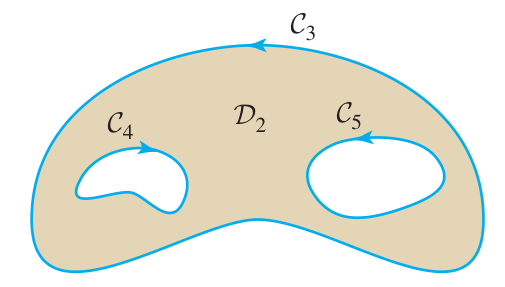
Some shapes have boundary lines on the inside. Do not forget to include these lines as part of the total boundary in Green’s Theorem! The orientation of these lines should be consistent with counter-clockwise circulation around infinitesimal boxes near the boundary. In the figure below, ${\mathcal{C}}_3$ and ${\mathcal{C}}_4$ are oriented correctly, while ${\mathcal{C}}_5$ has the wrong orientation. The boundary $\partial {\mathcal{D}}_2$ is therefore ${\mathcal{C}}_3+{\mathcal{C}}_4-{\mathcal{C}}_5$.