Theory

Introduction

The 2D version of a parametric curve is known as a parametric surface. Two parameters are needed to control the two independent dimensions of the surface. Component functions give the $(x,y,z)$ coordinates for each pair of values $(u,v)$:

$$\mathbf{r}(u,v)=(x(u,v),y(u,v),z(u,v)).$$

Introduction (part 2)

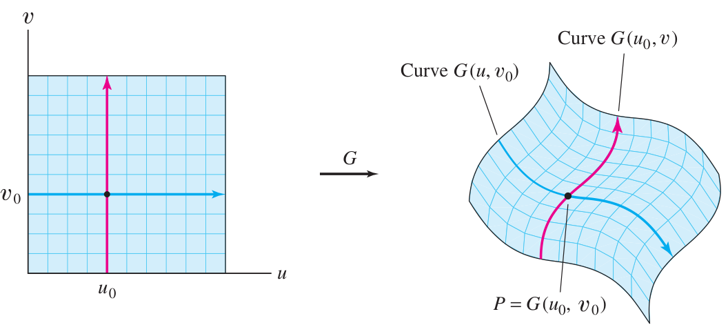
By holding $u=u_0$ constant or $v=v_0$ constant, one obtains grid curves. These correspond to trace curves when $\mathbf{r}(u,v)$ is the graph of a function, $\mathbf{r}=(u,v,f(u,v))$.

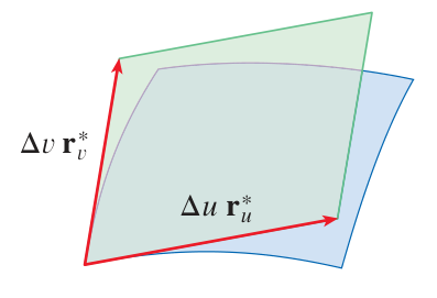
The two tangent vectors to the grid curves are computed by components, like the tangent vector of a parametric curve:

$$\begin{array}{rl}{\mathbf{r}}_u(u,v)& =\left(\frac{\partial x}{\partial u},\frac{\partial y}{\partial u},\frac{\partial z}{\partial u}\right),\\ {\mathbf{r}}_v(u,v)& =\left(\frac{\partial x}{\partial v},\frac{\partial y}{\partial v},\frac{\partial z}{\partial v}\right).\end{array}$$

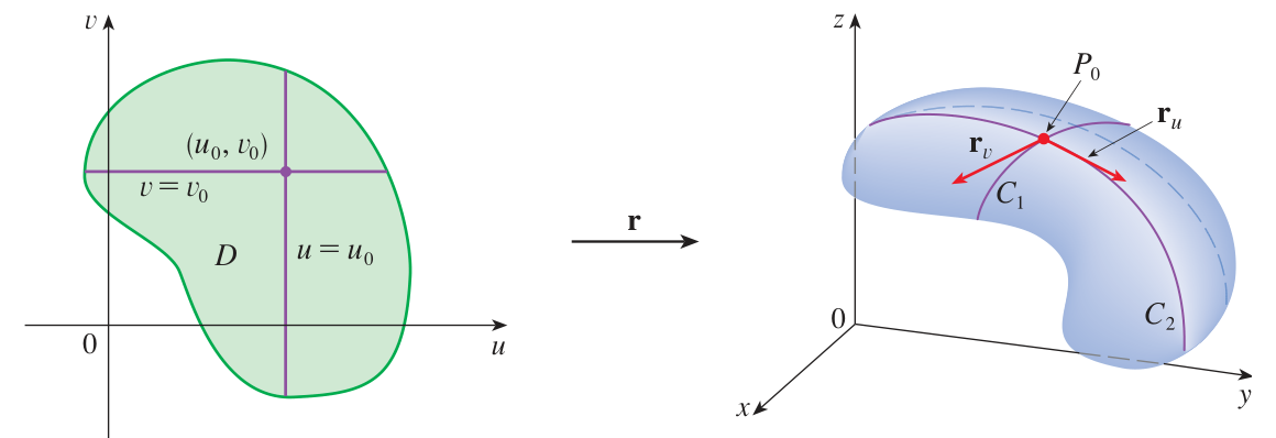
The tangent plane at a point on a surface given parametrically is given by taking all linear combinations of the tangent vectors added to the given starting point:

$${\mathbf{T}}_{(u,v)}(a,b)=\mathbf{r}(u,v)+a{\mathbf{r}}_u(u,v)+b{\mathbf{r}}_v(u,v),\text{fixed }(u,v),\text{ all }a,b\in \mathbb{R}.$$

The cross product $\mathbf{n}={\mathbf{r}}_u\times {\mathbf{r}}_v$ has several useful features:

• The direction of this cross product is normal to the tangent plane at the point $\mathbf{p}=\mathbf{r}(u,v)$. So the tangent plane could also be given in vector form by: $$\mathbf{n}\cdot ((x,y,z)-\mathbf{p})=0.$$
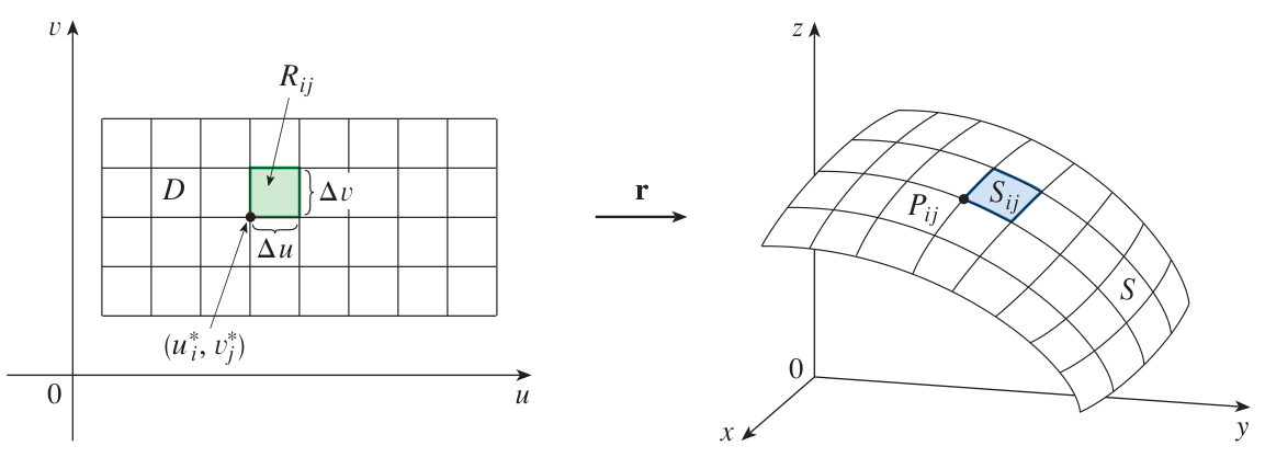
• The norm of this cross product gives a measure of area of the parallelogram created by ${\mathbf{r}}_u$ and ${\mathbf{r}}_v$, so: $$dA=|{\mathbf{r}}_u\times {\mathbf{r}}_v|dudv$$ gives the area of a microscopic region on the surface that corresponds to the area $dudv$ in the parameter space $(u,v)\in {\mathbb{R}}^2$. This formula is analogous to the formula $ds=|{\mathbf{r}}^{\prime }(t)|dt$ used to calculate the arc length distance along a curve.
  
  

Change of variables

Recall that we can calculate iterated integrals of a function $f(x,y)$:

$${\iint }_{\mathcal{D}}f(x,y)dxdy.$$

Such an integral can be interpreted as the volume (with sign) under the graph of $f(x,y)$.

Sometimes it is convenient to change variables before attempting to evaluate such an integral. This is a 2D analogue of $u$-substitution. Oftentimes in 2D it is useful to change variables to simplify the bounds, not just to simplify the integrand. For example, sometimes one can express the region $\mathcal{D}$ in terms of a rectangle in new coordinates, and compute the new integral as an iterated integral with constant bounds.

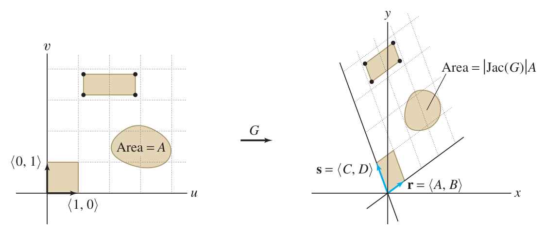
To change variables from $(x,y)$ to $(u,v)$, first substitute functions $x(u,v)$ and $y(u,v)$ in place of $x$ and $y$ inside $f(x,y)$. Next, consider that $\mathbf{r}(u,v)=(x(u,v),y(u,v),0)$ parametrizes the $xy$-plane using the new variables $(u,v)$. Then change the area element as follows:

$$dxdy=({\mathbf{r}}_u{\times }_z{\mathbf{r}}_v)dudv.$$

Sign included

This formula is essentially the same as the one we used for $dA$, except that we include the sign that comes with ${\mathbf{r}}_u{\times }_z{\mathbf{r}}_v$, leaving out the absolute value.

This is the analogue of $dx=u^{\prime }du$ in $u$-substitution, where if $x=-u$ then $dx=-du$. (Rather than $dx=|u^{\prime }|du$, which would produce $dx=du$.)

Notice that the order matters: if we swapped the role of $u$ and $v$, then ${\mathbf{r}}_u{\times }_z{\mathbf{r}}_v$ would gain a minus sign. This is a novel feature of signs in 2D that relates to geometry via the right-hand rule.

In this situation, the item ${\mathbf{r}}_u{\times }_z{\mathbf{r}}_v$ is also known as the Jacobian, or (when that name is used for the matrix itself), the Jacobian determinant:

$$\mathrm{Jac}(x,y)=\text{Jacobian}=\left|\begin{array}{cc}\frac{\partial x}{\partial u}& \frac{\partial x}{\partial v}\\ \frac{\partial y}{\partial u}& \frac{\partial y}{\partial v}\end{array}\right|=\frac{\partial x}{\partial u}\frac{\partial y}{\partial v}-\frac{\partial y}{\partial u}\frac{\partial x}{\partial v}.$$

Using this notation, we can rewrite the formula for change of variables:

$$\iint f(x,y)dxdy=\iint f(x(u,v),y(u,v))\mathrm{Jac}(x,y)dudv.$$

Surface integral - scalar

A scalar surface integral adds up the values of a function on a surface multiplied (locally) by elements of surface area on the surface. Given a surface $\mathcal{S}$ in ${\mathbb{R}}^3$ parametrized by $\mathbf{r}(u,v)$ (for $(u,v)\in \mathcal{D}$ with $\mathcal{D}$ some domain in the parameter space that maps to $\mathcal{S}$) and a scalar function $f(x,y,z)$, we can compute a surface integral of $f$ over $\mathcal{S}$ with the formula:

$${\iint }_{\mathcal{S}}f(x,y,z)dA={\iint }_{\mathcal{D}}f(\mathbf{r}(u,v))|{\mathbf{r}}_u\times {\mathbf{r}}_v|dudv.$$

This formula is the 2D analogue of the formula for a scalar line integral: ${\int }_{\mathcal{C}}fds={\int }_a^{b}f(\mathbf{r}(t))|{\mathbf{r}}^{\prime }(t)|dt$.

Surface integral - vector - flux across

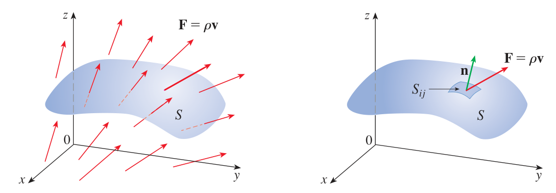
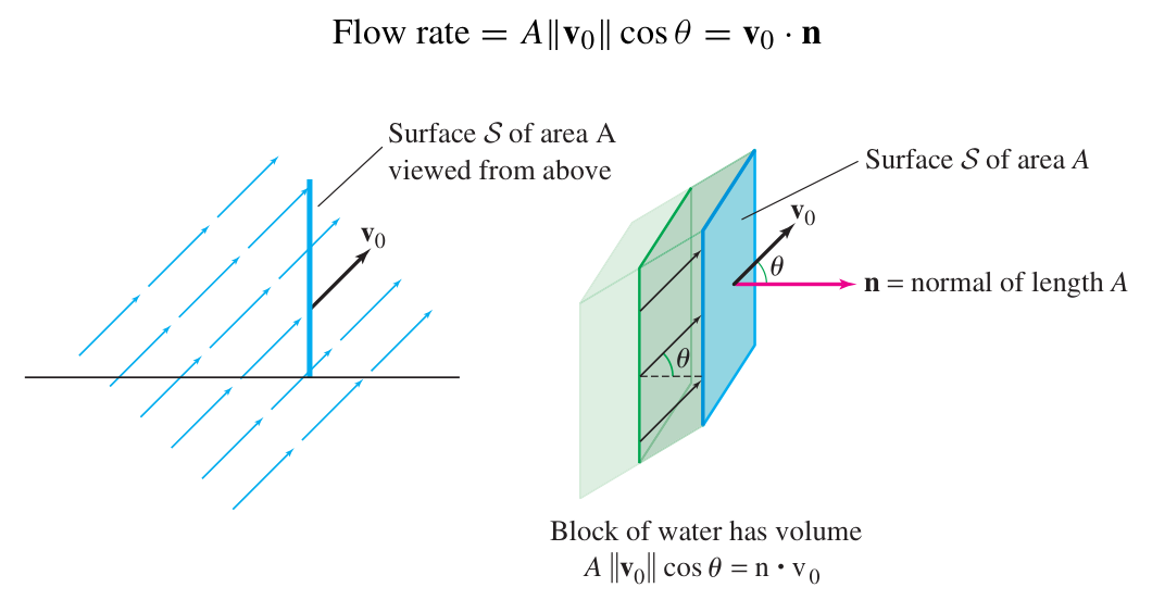
A vector surface integral adds up the total amount that a vector field $\mathbf{F}$ crosses a surface $\mathcal{S}$. This total is called the flux across $\mathcal{S}$. When $\mathbf{F}=\mathbf{v}$ is the velocity vector field of a fluid flow, the flux quantifies the total rate of flow crossing the surface. It is defined like the ‘across’ line integral, but instead of ${\mathbf{e}}_{\mathbf{n}}$ derived from a rotation $\mathbf{n}$ of the tangent vector ${\mathbf{r}}^{\prime }$, we use ${\mathbf{e}}_{\mathbf{n}}$ derived from the normal vector to the surface, $\mathbf{n}={\mathbf{r}}_u\times {\mathbf{r}}_v$. In terms of a parametrization $\mathbf{r}(u,v)$ of the surface $\mathcal{S}$, it is computed using the formula:

$${\iint }_{\mathcal{S}}\mathbf{F}\cdot d\mathbf{A}={\iint }_{\mathcal{S}}\mathbf{F}\cdot {\mathbf{e}}_{\mathbf{n}}dA={\iint }_{\mathcal{D}}\mathbf{F}(\mathbf{r}(u,v))\cdot \mathbf{n}(u,v)dudv.$$

Here $d\mathbf{A}$ is a vector with length $dA$ and direction $\mathbf{n}$, normal to the surface. So $d\mathbf{A}={\mathbf{e}}_{\mathbf{n}}dA=\mathbf{n}dudv$ because $|{\mathbf{r}}_u\times {\mathbf{r}}_v|{\mathbf{e}}_{\mathbf{n}}=\mathbf{n}$. This is analogous to $\mathbf{F}\cdot {\mathbf{e}}_{\mathbf{n}}ds=\mathbf{F}\cdot \mathbf{n}dt$ in the ‘across’ line integral.

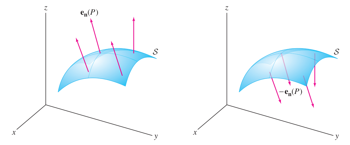
As with line integrals, the sign of the vector surface integral depends on the orientation of the surface. In 2D the orientation is the direction of $\mathbf{n}$. This direction comes from the cross product ${\mathbf{r}}_u\times {\mathbf{r}}_v$ and thus it depends on the order of $u$ and $v$, as well as the sign of each of them. (Exchanging $u$ and $v$, or setting $u\mapsto -u$, switches the direction of $\mathbf{n}$.)

Surface integral - vector - flux across (part 2)

Physical Application: Faraday’s Law of Induction [optional]

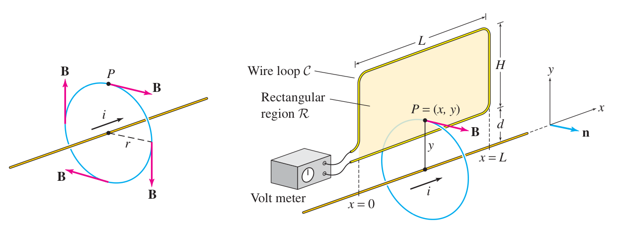
Faraday’s Law of Induction states that the ‘aligned’ vector line integral of electric field around a curve $\mathcal{C}$ is proportional to the rate of change of magnetic flux through the surface $\mathcal{S}$ enclosed by $\mathcal{C}$:

$${\int }_{\mathcal{C}}\mathbf{E}\cdot d\mathbf{s}=-\frac{d}{dt}{\iint }_{\mathcal{S}}\mathbf{B}\cdot d\mathbf{A}.$$

Given a formula for the current $I(t)$ flowing in the linear wire, one computes the magnetic field $\mathbf{B}$ in the region above the linear wire. By integrating $\mathbf{B}$ over $\mathcal{S}$, one obtains the total flux as a function of time; taking the (negative of the) derivative gives the quantities in the Faraday identity above. Because $\mathbf{E}=\nabla V$ for the voltage $V(x,y,z)$, the value of the line integral on the LHS is actually the voltage drop around the wire $\mathcal{C}$ (by the FT of Line Integrals).