Theory

Examples of differential equations

The next examples illustrate what some important differential equations look like. Some other matters come up too, for example that solutions to differential equations are functions (not numbers), and that a single equation can have many solutions.

Legendre’s equation:

$$(1-x^2)\frac{d^{2}y}{d{x}^2}-2x\frac{dy}{dx}+n(n+1)y=0.$$

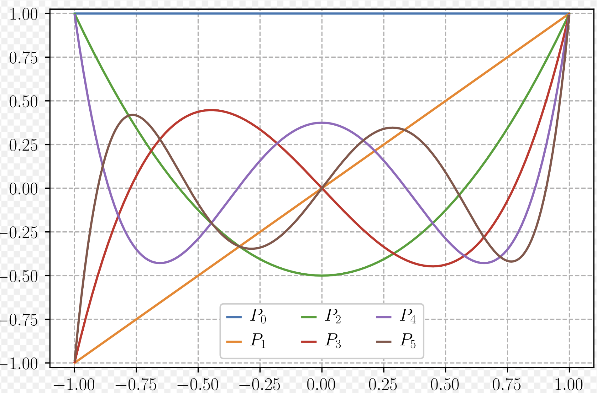
The solution to this equation is a polynomial $y=P_n(x)$ for each $n$. The first few polynomials are:

$n$	$P_n(x)$
0	1
1	$x$
2	$\frac{1}{2}(3x^2-1)$
3	$\frac{1}{2}(5x^3-3x)$

These polynomials have many useful properties. Their most important property is “orthogonality”:

$${\int }_{-1}^{+1}{P}_n(x)P_m(x)dx=0\text{ unless }n=m.$$

Bessel’s equation:

$$x^2\frac{d^{2}y}{d{x}^2}+x\frac{dy}{dx}+(x^2-{\alpha }^2)y=0.$$

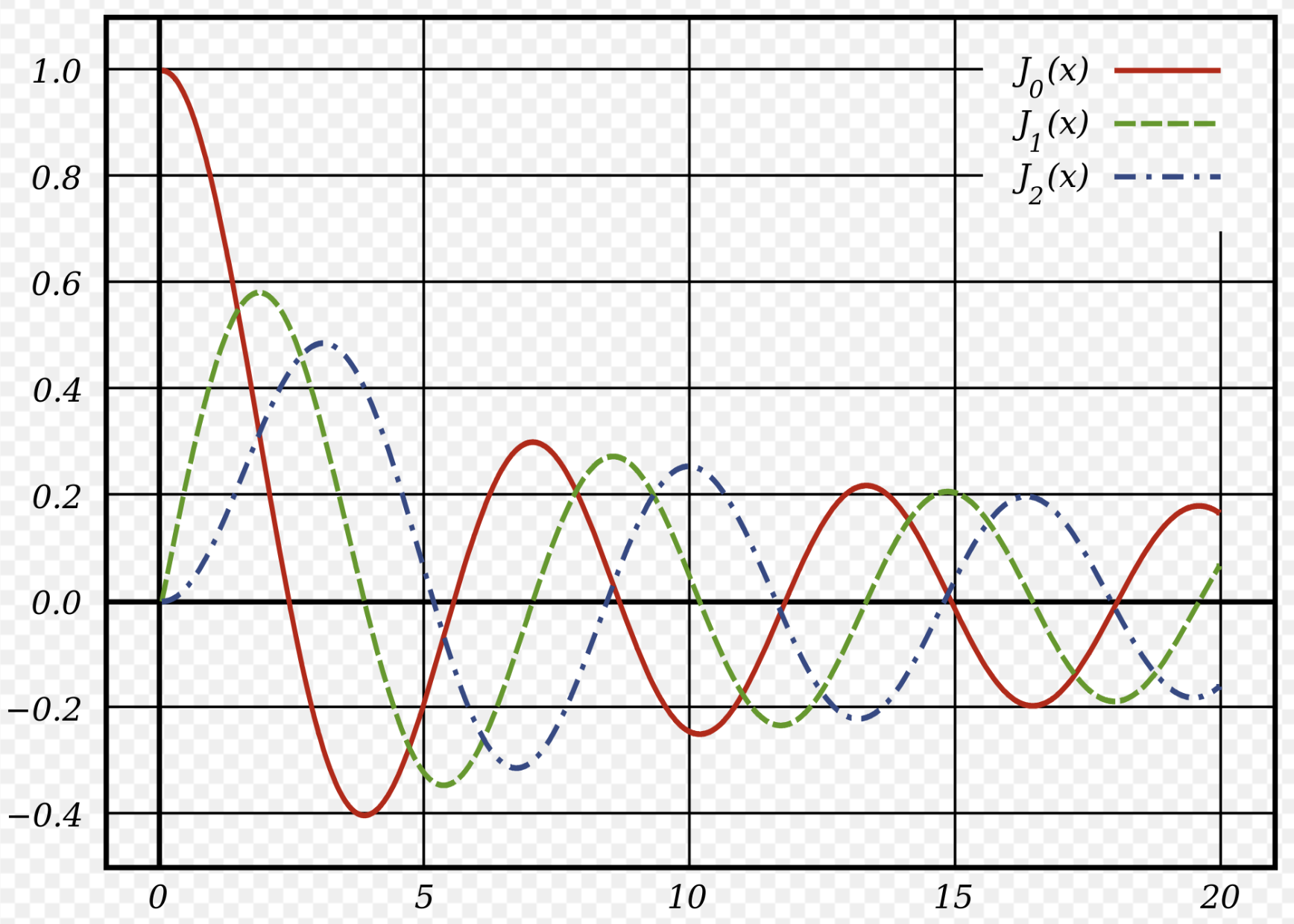
Solutions to this equation are used to study heat conduction and waves (electromagnetic or quantum wavefunctions).

Airy’s equation:

$$\frac{d^{2}y}{d{x}^2}-xy=0.$$

The solution to Airy’s equation arises in quantum mechanics, optics, and probability.

Chebyshev’s equation:

$$(1-x^2)y^{\prime \prime }-x{y}^{\prime }+p^{2}y=0.$$

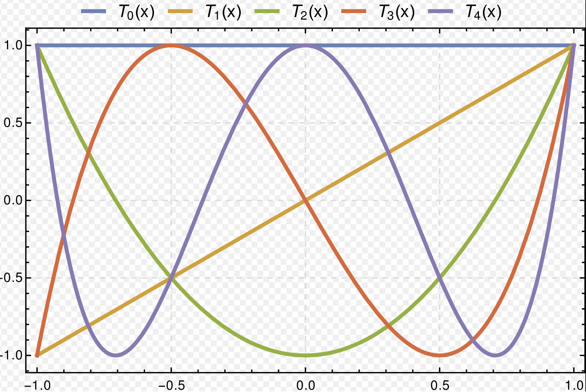
Solutions to this equation give polynomials $T_n(x)$ and $U_n(x)$ that describe the higher sum rules of trig functions:

$$\begin{array}{rl}\cos (n\theta )& =T_n(\cos (\theta ))\\ \sin (n\theta )& =\sin (\theta )U_{n-1}(\cos (\theta )).\end{array}$$

Hermite’s equation:

$$y^{\prime \prime }-2x{y}^{\prime }+2py=0.$$

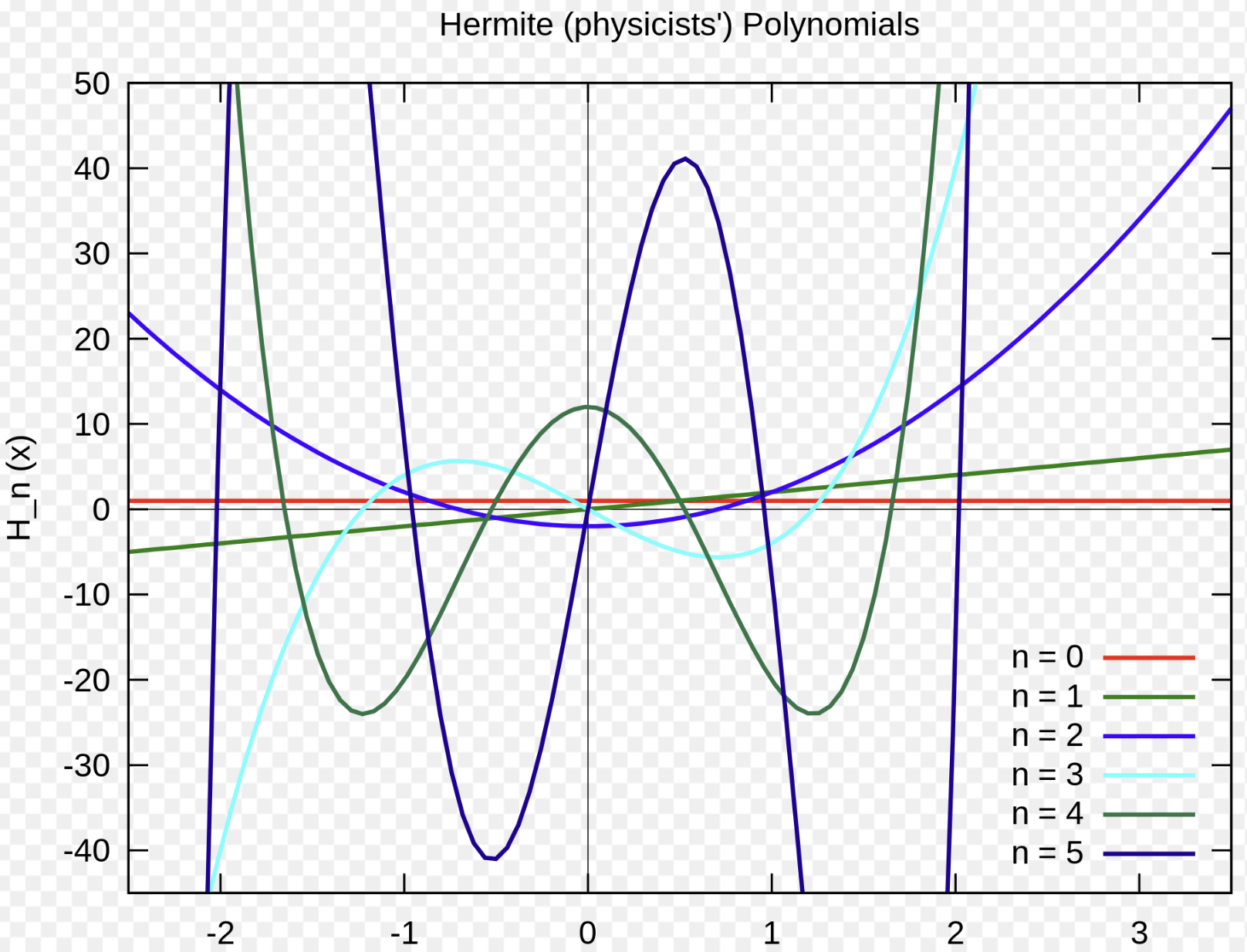
Solutions to this equation are used in quantum mechanics, signal processing, numerical analysis, and probability.

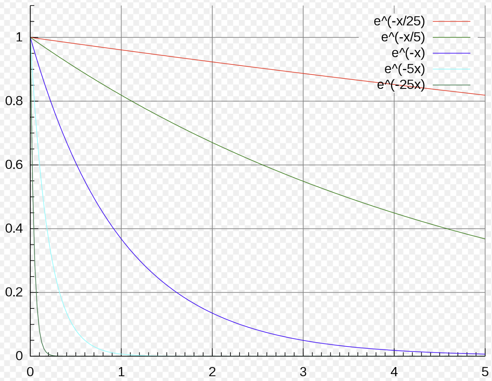
Exponential decay:

$$\frac{dy}{dx}-ky=0.$$

This equation models countless physical processes.

Concepts of differential equations

What we typically mean by a “differential equation” is a function $F$ of, say, $n+2$ variables, that is given by some algebraic expression (possibly involving trig or exponential functions as well). A solution to the equation is a function $y(x)$ with the property that:

$$F\left(x,y(x),y^{\prime }(x),y^{\prime \prime }(x),\dots ,y^{(n)}(x)\right)=0$$

for all $x$. The order $n$ of the differential equation is the order of the highest derivative that appears in the expression for $F$.

A differential equation is called explicit when it can be written with the highest derivative isolated, on the other side:

$$F(x,y,y^{\prime },\dots ,y^{(n-1)})=y^{(n)}.$$

Sometimes a differential equation is “solved” by finding an equation relating $y$ and $x$ which cannot be solved explicitly for $y$ in terms of $x$. In this situation, a (connected) set of points $(x,y)$ satisfying the solution equation is called an integral curve of the differential equation.

Ordinary differential equations involve only ordinary derivatives, while partial differential equations involve partial derivatives.

Usually we assume that $F$ is a familiar kind of function that is constructed using algebraic operations (possibly with trig or exponential functions) applied to the arguments.

There is a fundamental distinction between linear and nonlinear differential equations. A linear differential operator is a linear function taking functions to functions. For example:

$$\left(\frac{d^2}{d{x}^2}-x\right):y(x)⟼\frac{d^{2}y}{d{x}^2}-xy.$$

Concepts of differential equations (part 2)

Linear differential equations are defined as those corresponding to a linear differential operator. (By applying the operator to $y$ and setting the result equal to some function.) Roughly speaking, this means they are equations in which $y,y^{\prime },y^{\prime \prime },\dots$ can appear only to the first power.