Theory

Introduction

The $1$D scalar wave equation is:

$$\frac{{\partial }^{2}y}{\partial t^2}=v^2\frac{{\partial }^{2}y}{\partial x^2}$$

for some constant $v$ and function $y(x,t)$ that depends on position $x$ and time $t$.

If $y(x,t)$ describes the vertical displacement of a rubber band, then $y(x,t)$ will (to good approximation) satisfy the wave equation.

Many physical systems satisfy this equation to some degree of approximation. There are higher dimensional analogues as well. For example in $3$D the wave equation looks like this:

$$\frac{{\partial }^{2}u}{\partial t^2}=v^2\left(\frac{{\partial }^{2}u}{\partial x^2}+\frac{{\partial }^{2}u}{\partial y^2}+\frac{{\partial }^{2}u}{\partial z^2}\right).$$

Some fields $u(t,x,y,z)$ that satisfy the $3$D wave equation include:

• Density of air (sound waves).
• Each vector component of the electric or magnetic field.

An extremely important property of the wave equation is linearity. Given any two solutions $y_1(x,t)$ and $y_2(x,t)$ to the wave equation, any linear combination of them:

$$y(x,t)=c_1{y}_1(x,t)+c_2{y}_2(x,t)$$

is also a solution. In physical settings, linearity implies the superposition principle that we have discussed before. In addition to its physical interest, superposition has a practical consequence: solutions to the wave equation can be broken into sums (or infinite series) of well-behaved solutions, meaning waves that are easy to describe, analyze, and visualize.

In this section we focus on the $1$D scalar wave equation. We will study it from two points of view: traveling waves and standing waves. The former are sometimes just called waves, and the latter are sometimes called normal modes or simply modes for short.

These points of view correspond to wave decompositions. Traveling waves preserve a shape function as they move through space. Thinking in terms of traveling waves enables the study of energy transmission, reflections, and media interfaces. Standing waves lead to simplification of a different sort. They satisfy separation of variables which in turn leads to sinusoidal terms with nodes and peaks that are fixed in space. These sinusoids are independent of each other. They interact nicely with Fourier series.

For the rest of the section we return to the scalar wave equation, $\frac{{\partial }^{2}y}{\partial t^2}=v^2\frac{{\partial }^{2}y}{\partial x^2}$.

Traveling waves

A traveling wave $y(x,t)$ is given by a function of a linear combination of space and time:

$$y(x,t)=F(x+at).$$

At any given fixed $t$, the ‘shape’ of the solution $y$ across the $x$ variable is described by the same shape function $F$, but with a horizontal shift given by $at$.

Traveling waves $y=F(x+at)$ satisfy the wave equation, for any shape function $F$, when $a=\pm v$:

Traveling waves (part 2)

Conversely, d’Alembert discovered an argument that essentially all solutions to $\frac{{\partial }^{2}y}{\partial t^2}=v^2\frac{{\partial }^{2}y}{\partial x^2}$ are given by a sum of traveling waves, with one term traveling leftwards, and another term traveling rightwards:

Wave equation solutions are traveling waves

Suppose $y(x,t)$ has all requisite partial derivatives, and it satisfies the wave equation $\frac{{\partial }^{2}y}{\partial t^2}=v^2\frac{{\partial }^{2}y}{\partial x^2}$.

Then $y(x,t)=\ell (x+vt)+r(x-vt)$ for some $\ell (u)$ and $r(u)$ shape functions.

Derivation of d’Alembert’s solution

Let us change variables to $p=x+vt$ and $q=x-vt$. Then:

$$\begin{array}{rl}\frac{\partial y}{\partial x}& =\frac{\partial y}{\partial p}\frac{\partial p}{\partial x}+\frac{\partial y}{\partial q}\frac{\partial q}{\partial x}\\ & =\frac{\partial y}{\partial p}+\frac{\partial y}{\partial q},\\ & \\ \frac{{\partial }^{2}y}{\partial x^2}& =\frac{{\partial }^{2}y}{\partial p^2}\frac{\partial p}{\partial x}+\frac{{\partial }^{2}y}{\partial q\partial p}\frac{\partial q}{\partial x}+\frac{{\partial }^{2}y}{\partial p\partial q}\frac{\partial p}{\partial x}+\frac{{\partial }^{2}y}{\partial q^2}\frac{\partial q}{\partial x}\\ & =\frac{{\partial }^{2}y}{\partial p^2}+2\frac{{\partial }^{2}y}{\partial p\partial q}+\frac{{\partial }^{2}y}{\partial q^2},\end{array}$$

and:

$$\begin{array}{rl}\frac{\partial y}{\partial t}& =\frac{\partial y}{\partial p}\frac{\partial p}{\partial t}+\frac{\partial y}{\partial q}\frac{\partial q}{\partial t}\\ & =v\frac{\partial y}{\partial p}-v\frac{\partial y}{\partial q},\\ & \\ \frac{{\partial }^{2}y}{\partial t^2}& =v^2\frac{{\partial }^{2}y}{\partial p^2}-v^2\frac{{\partial }^{2}y}{\partial q\partial p}-v^2\frac{{\partial }^{2}y}{\partial p\partial q}+v^2\frac{{\partial }^{2}y}{\partial q^2}\\ & =v^2\left(\frac{{\partial }^{2}y}{\partial p^2}+\frac{{\partial }^{2}y}{\partial q^2}\right)-2v^2\frac{{\partial }^{2}y}{\partial p\partial q}.\end{array}$$

It follows that the wave equation is equivalent to the equation:

$$\frac{{\partial }^{2}y}{\partial p\partial q}=0.$$

Now we can integrate this equation in $p$ and then in $q$:

$$\begin{array}{rl}\int \frac{{\partial }^{2}y}{\partial p\partial q}dp=0& ⇝⇝\frac{\partial y}{\partial q}=f(q)\\ & \\ & \int \frac{\partial y}{\partial q}dq=\int f(q)dq⇝⇝y=F(q)+G(p).\end{array}$$

Here $f(q)$ is introduced as a constant of the $p$ integration, $F$ is an antiderivative (so $F^{\prime }=f$), and $G(p)$ is a constant of the $q$ integration.

Then by plugging in $q=x+vt$ and $p=x-vt$ we obtain:

$$y(x,t)=F(x+vt)+G(x-vt).$$

Standing waves

Waves that do not travel laterally are called standing waves. This lack of lateral motion may be described mathematically by specifying a fixed shape function $F(x)$; the standing wave is then described by $y(x,t)=a(t)F(x)$ where the amplitude $a(t)$ depends on time, but at any given time, the shape of the wave across space (ignoring the amplitude) is $F(x)$. In many applied contexts, standing waves are called normal modes or simply modes.

Let us find the normal modes of the $1$D wave equation. These are solutions of the form $y(x,t)=a(t)F(x)$. From this it follows that $y_{xx}=a(t)F^{\prime \prime }(x)$ and $y_{tt}=a^{\prime \prime }(t)F(x)$. The wave equation then dictates:

$$a^{\prime \prime }(t)F(x)=v^{2}a(t)F^{\prime \prime }(x)$$

which implies

$$\frac{1}{v^2}\frac{a^{\prime \prime }(t)}{a(t)}=\frac{F^{\prime \prime }(x)}{F(x)}.$$

The left side does not depend on $x$, and the right side does not depend on $t$. Equality of the sides implies that both sides equal some constant $-\lambda$. (Adding the minus sign for future convenience.)

So we end up two second order equations that are completely independent:

$$\begin{array}{rl}{a}^{\prime \prime }+v^2\lambda a& =0\\ F^{\prime \prime }+\lambda F& =0.\end{array}$$

The solutions when $-\lambda <0$ are sinusoids with frequency ratio $v$:

$$\begin{array}{rl}a(t)& =A\cos (v\sqrt{\lambda }t+\varphi ),\\ F(x)& =B\cos (\sqrt{\lambda }x+\psi ).\end{array}$$

In the absence of boundaries, these solutions can occur with any frequency.

Free standing waves can be related to traveling waves by rewriting the product with the trig identity $2\cos (A)\cos (B)=\cos (A+B)+\cos (A-B)$:

$$\begin{array}{rl}y(x,t)& =AB\cos (v\sqrt{\lambda }t+\varphi )\cos (\sqrt{\lambda }x+\psi )\\ & =\frac{AB}{2}\cos (\sqrt{\lambda }(x+vt)+\varphi +\psi )+\frac{AB}{2}\cos (\sqrt{\lambda }(x-vt)+\varphi -\psi ).\end{array}$$

These are waves traveling with velocity $v$, to the left and the right respectively, with the same amplitude. “Interference” of the traveling waves is equivalent to the presentation as standing waves.
https://en.wikipedia.org/wiki/Standing_wave#/media/File:Waventerference.gif

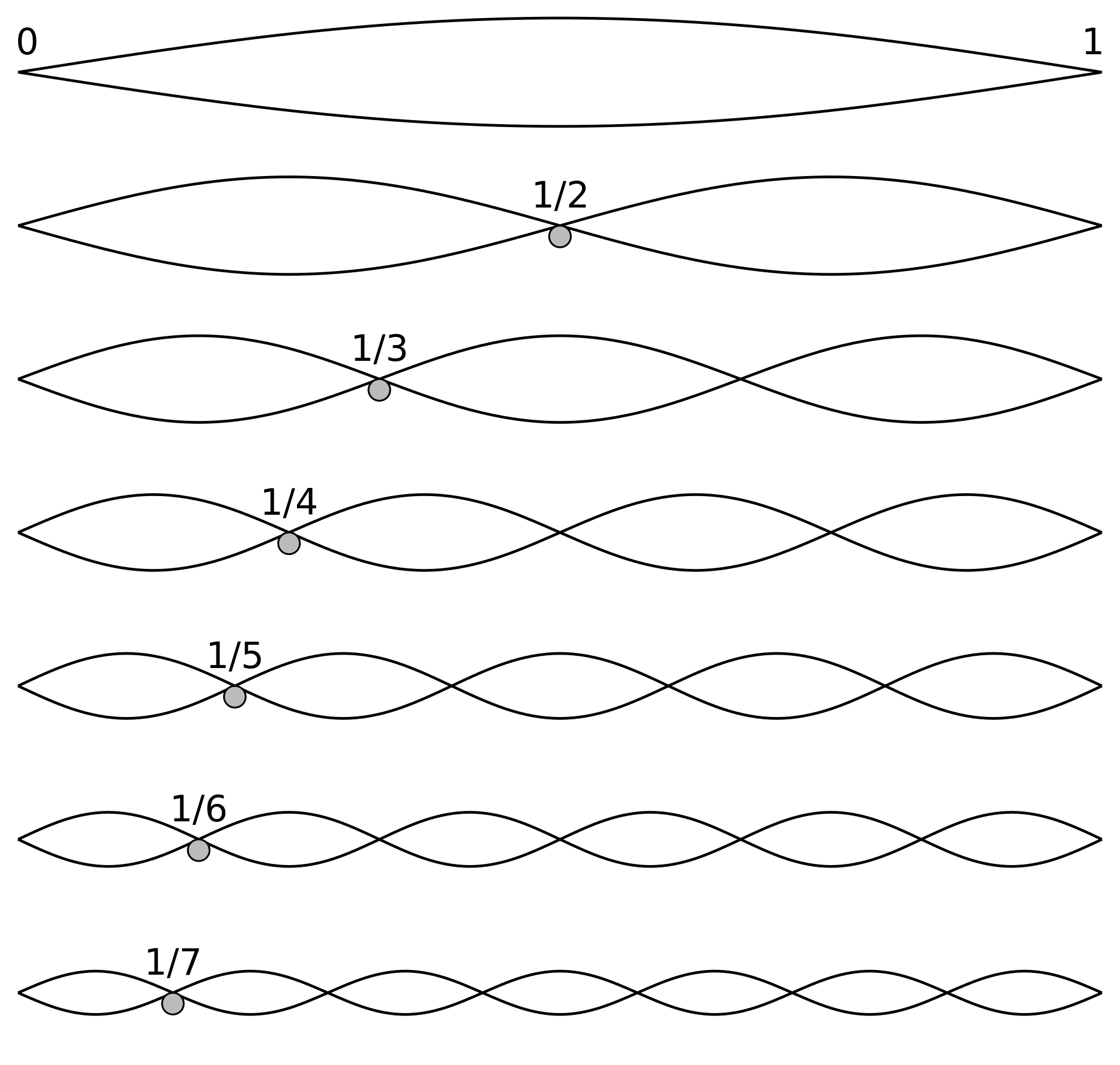
Standing waves have a natural significance in the context of boundary value problems where the normal modes frequently receive a large contribution of the energy of natural vibrations. The boundary conditions have the effect of allowing only certain discrete values of $\lambda$, which is a kind of quantization phenomenon.

Suppose a vibrating rubber band satisfies the wave equation $v^2\frac{{\partial }^{2}y}{\partial x^2}=\frac{{\partial }^{2}y}{\partial t^2}$ and boundary conditions $y(0,t)=0=y(L,t)$. The natural mode solutions to this BVP are given by $u_n(x,t)=\cos (\frac{n\pi }{L}vt)\sin (\frac{n\pi }{L}x)$.

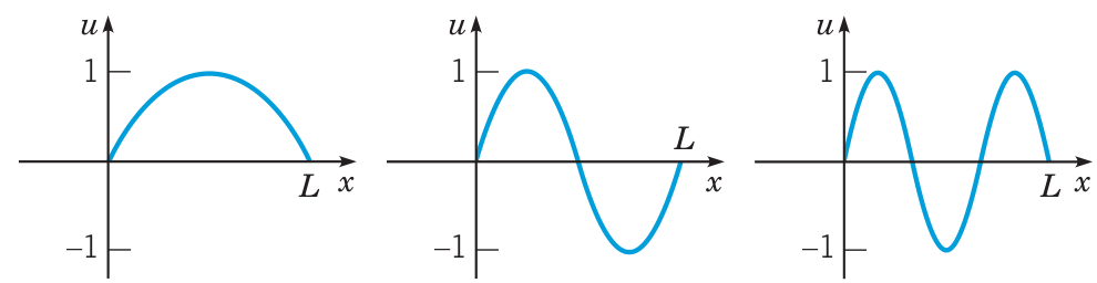
https://en.wikipedia.org/wiki/Standing_wave#/media/File:Standing_waves_on_a_string.gif