Theory

Introduction

Recall the inversion problems we are interested in, namely solving for vector $\mathbf{x}$ or matrix $X$ in these equations:

$$A\mathbf{x}=\mathbf{b},AX=B.$$

The LU factorization, and in particular the row reduction process yielding row-echelon form, is the perfect tool to solve these equations. Replacing $A$ with $LU$, we have:

$$LU\mathbf{x}=\mathbf{b},LUX=B.$$

In the process of finding $LU$ we actually found $L^{-1}=L_n^{-1}\cdots L_1^{-1}$. Applying the $L^{-1}$ action to both sides:

$$U\mathbf{x}={\mathbf{b}}^{\prime },UX=B^{\prime }$$

where ${\mathbf{b}}^{\prime }=L^{-1}\mathbf{b}$ and $B^{\prime }=L^{-1}B$.

Now assume that $U$ is in row-echelon form. We can solve these equations for $\mathbf{x}$ and $X$ using the second fundamental technique, called back substitution.

Just as elimination is equivalent to inverting $L$, back substitution is equivalent to inverting $U$. Inverting $L$ with eliminations provides the row-echelon form, and inverting $U$ with back substitutions provides the reduced row-echelon form.

Reduced row-echelon form

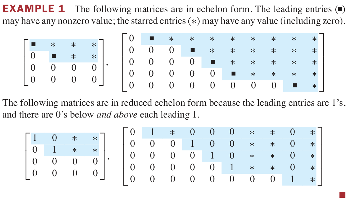
Given $U$ in row-echelon form, it is also in reduced row-echelon form (RREF) when the leading nonzero entries in each row are ones, and any column with a leading one has all other entries equal to zero.

Back substitution is the process of applying row-scale and row-add matrix actions to convert a matrix in REF to a matrix in RREF. This is a continuation of “row reduction,” with a difference being that the matrices performing back substitution operations are not lower triangular, they are now upper triangular. Another difference is that we don’t have good reasons (in terms of applications) to record these back substitution matrices, we simply let them act on our matrix, or simultaneously on our matrix and vector (in the case of $A\mathbf{x}=\mathbf{b}$) or on our matrix and matrix (in the case of $AX=B$).

To find the RREF of a matrix in REF, we:

Computing reduced row-echelon form from row-echelon form

• Act by row-scale matrices to change the leading entries to ones.
• Act by more row-add matrices to eliminate the entries above leading ones.

Any RREF matrix can be written in terms of block submatrices:

$$\left(\begin{array}{cc}{I}_k& X\\ 0& 0\end{array}\right).$$

Here $I_k$ is the identity as a submatrix (the size of $k$ depends on how many zeros are in $U$), $X$ is some other submatrix, and $\begin{array}{cc}0& 0\end{array}$ are zeros filling out the rest of $U$.

Preimage of a vector

The RREF of a matrix reveals the complete set of possible inverses (preimages) of a given vector.

Preimage of a vector (part 2)

If we wish to solve an equation $A\mathbf{x}=\mathbf{b}$ and $A$ is not yet in reduced row-echelon form, then we must convert $A$ to that form, while simultaneously applying the row reductions and pivots to the vector $\mathbf{b}$. (This means applying the same invertible transformations to both sides of the equation.) Row reduction is easily performed on $A$ and $\mathbf{b}$ simultaneously by combining them into the augmented matrix $\left(\begin{array}{rr}A& \mathbf{b}\end{array}\right)$ and row reducing this instead. (This means: create a matrix by adding $\mathbf{b}$ as an additional column to $A$, and put a vertical line between them to demarcate the end of $A$.)

Solving linear systems

A linear system looks something like this:

$$\begin{array}{rl}{x}_1-2x_2+x_3& =0\\ 2x_2-8x_3& =8\\ 5x_1-5x_3& =10.\end{array}$$

This system is easily represented as the vector inversion problem of $A\mathbf{x}=\mathbf{b}$, with $\mathbf{x}=(x_1,x_2,x_3)$ and $\left(\begin{array}{rr}A& \mathbf{b}\end{array}\right)$ given by:

$$\left(\begin{array}{rr}A& \mathbf{b}\end{array}\right)=\left(\begin{array}{rrrr}1& -2& 1& 0\\ 0& 2& -8& 8\\ 5& 0& -5& 10\end{array}\right)$$

The techniques of elimination and back substitution that we have learned for matrices correspond to the techniques of the same names that you already know for solving systems of equations.

Preimage of a matrix

The technique for inverting a vector can be applied to find the preimage of a matrix simply by inverting the column vectors of that matrix. Namely, given the equation:

$$AX=B,$$

notice that if we write $X$ and $B$ in terms of their column vectors, we have:

$$\begin{array}{c}A\left(\begin{array}{cccc}{\mathbf{x}}_1& {\mathbf{x}}_2& \dots & {\mathbf{x}}_n\end{array}\right)=\left(\begin{array}{cccc}{\mathbf{b}}_1& {\mathbf{b}}_2& \dots & {\mathbf{b}}_n\end{array}\right)\\ A{\mathbf{x}}_1={\mathbf{b}}_1,A{\mathbf{x}}_1={\mathbf{b}}_1,\dots ,A{\mathbf{x}}_n={\mathbf{b}}_n.\end{array}$$

In principle, we can simply invert ${\mathbf{b}}_1,\dots ,{\mathbf{b}}_n$ one at a time, in sequence.

In practice, a much faster way to find $X$ is to write the augmented matrix $\left(\begin{array}{rr}A& B\end{array}\right)$ and row reduce this matrix.

The most important use of this technique is to find the inverse of an invertible matrix. Given $A$, the inverse $A^{-1}$ is found by computing the preimage of $I_n$ under the action of $A$, in other words by setting $B=I_n$ and row reducing the augmented matrix $\left(\begin{array}{rr}A& I_n\end{array}\right)$.