Theory

Introduction

These techniques work well if the given data happens to lie near a lower-dimensional vector subspace or submanifold of the original space.

Foundational algorithms are

• PCA “principle component analysis” — vector subspaces
  • starts with $X\subset {\mathbb{R}}^n$ a finite metric space (point-cloud data)
• MDS “multidimensional sampling” — manifold subspaces
  • starts with arbitrary metric space $(X,d)$

Goal:

Given (small) $k\in {\mathbb{Z}}_{\ge 0}$, find an optimal map $\theta :X\to {\mathbb{R}}^k$ which in some sense represents the structure of the data by minimizing the error:

$$\mathcal{E}=\sum _{x_i,x_j\in X}(d_X(x_i,x_j)-d_{{\mathbb{R}}^k}(\theta (x_i),\theta (x_j)){)}^2$$

PCA

Let $M$ be an $n\times n$ matrix with eigenvalues ${\lambda }_i$ and eigenvectors ${\mathbf{v}}_i$, so $M{\mathbf{v}}_i={\lambda }_i{\mathbf{v}}_i$.

Recall that if $M$ is symmetric, we know that ${\lambda }_i\in \mathbb{R}$ and

$${\lambda }_i\ne {\lambda }_j⟹{\mathbf{v}}_i\perp {\mathbf{v}}_j$$

For PCA, we start with $X=\{{\mathbf{x}}_1,{\mathbf{x}}_2,\dots ,{\mathbf{x}}_3\}\subset {\mathbb{R}}^n$. Fix $k\in {\mathbb{Z}}_{\ge 0}$ small.

The goal is to find an “optimal” linear map $\theta :{\mathbb{R}}^n\to {\mathbb{R}}^k$ which distorts distances between data points as little as possible. (Minimal mean-square error.)

PCA Algorithm:
(1) Normalization

Consider $\mu =\frac{1}{n}{\sum }_i{\mathbf{x}}_i$ and let ${\tilde{\mathbf{x}}}_i={\mathbf{x}}_i-\mu$.

(2) Covariance matrix

Define the covariance matrix $C$:

$$C=\frac{1}{n}\sum _i{\tilde{\mathbf{x}}}_i{\tilde{\mathbf{x}}}_i^{\mathsf{T}}$$

Note that $C_{jk}={\mathbf{x}}_j\cdot {\mathbf{x}}_k$. Then, since each summand of $C$ is symmetric, $C$ must be symmetric.

(3) Eigenvalues

Compute the top (largest) $k$ eigenvalues of $C$.

If these are pairwise distinct, the corresponding eigenvectors are all linearly independent, so they span a $k$-dimensional linear subspace $V$.

Consider the orthogonal projection $\theta :{\mathbb{R}}^n\to V$.

(Note: one must somehow identify $V$ with ${\mathbb{R}}^k$ first.)

If some eigenvalue ${\lambda }_j$ has multiplicity, then consider the corresponding eigenspace $V_j$.

Theorem:

The outcome of this algorithm is an optimal $\theta$ which minimizes the error $\mathcal{E}$.

(In the context of PCA or MDS, in fact.)

Combining techniques

It is often reasonable to combine techniques discussed thus far.

For example, the outcome of PCA/MDS may be fed into Mapper; a coordinate project in the PCA output may be used as the filter function.

MDS

Multi-dimensional scaling starts with an arbitrary finite metric space $(X,d)$, and attempts to embed this in ${\mathbb{R}}^k$ in a way that is optimal in the sense of minimizing $\mathcal{E}$. This is done as follows:

(1) Metric matrix:

$$D_{ij}=d_X({\mathbf{x}}_i,{\mathbf{x}}_j)$$

(2) $H$ and $Z$

Let $H$ be the matrix $H=I-\frac{1}{n}1$ where $1$ is the matrix with all entries $1$.

Let $Z$ be the matrix $Z=-\frac{1}{2}HDH$.

(This step centers the result at the origin.)

(3) Define $\theta :X\to {\mathbb{R}}^k$:

Create a matrix $A$ with columns the eigenvectors ${\mathbf{v}}_j$, normalized so that $||{\mathbf{v}}_j|{|}^2={\lambda }_j$. Then:

$$\theta (x_i)=i^{\text{th}}\text{ row of }{A}^{\mathsf{T}}$$

Isomap manifold learning

The given data is aligned along a non-linear subspace of ${\mathbb{R}}^n$.

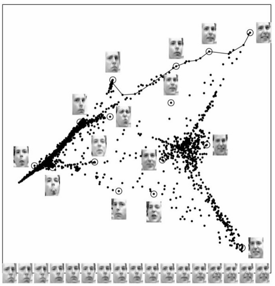
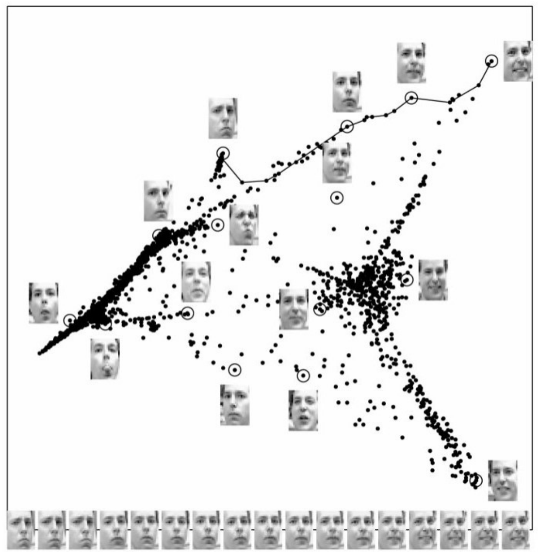
This method is used in facial recognition, for example.

We are assuming that the data lies along (very near) a submanifold $M\subset {\mathbb{R}}^n$. This $M$ is assumed to have an “intrinsic” metric $d_M(x,y)$ for $x,y\in M$.

$$d_M(x,y)=\underset{\text{curves }\alpha }{\min }{\int }_0^1||\dot{\alpha }(t)||dt$$

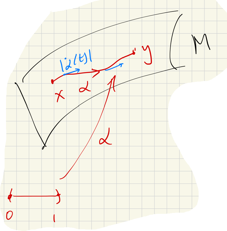
The idea of isomap is that, assuming $M\subset {\mathbb{R}}^n$ is smoothly embedded, there is a scale at which

$$d_M(x,y)\sim d_{{\mathbb{R}}^n}(x,y)$$

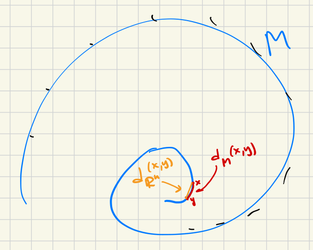
Isomap description in detail:

Let us be given $X=\{{\mathbf{x}}_1,\dots ,{\mathbf{x}}_m\}\subset {\mathbb{R}}^n$, as well as a scale $\epsilon >0$ and a target dimension $k$.

Isomap procedure

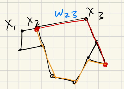
(1) Build weighted graph $G$:

• Vertices: the points ${\mathbf{x}}_1,\dots ,{\mathbf{x}}_m$
• Edges: join ${\mathbf{x}}_i$ to ${\mathbf{x}}_j$ when $d({\mathbf{x}}_i,{\mathbf{x}}_j)<\epsilon$
• Weights: the distances $w_{ij}=d({\mathbf{x}}_i,{\mathbf{x}}_j)$

(2) New metric space $(X^{\prime },d_{X^{\prime }})$:

Same points, new distances:

$$d_{X^{\prime }}({\mathbf{x}}_i,{\mathbf{x}}_j)=\underset{\begin{array}{c}\text{paths }{\mathbf{x}}_i\\ \text{ to }{\mathbf{x}}_j\text{ in }G\end{array}}{\min }\sum \text{path weight}$$

(Use Dijkstra’s Algorithm to compute the minimal path.)

(3) Apply PCA/MDS:

Find an optimal map $\theta :X^{\prime }\to {\mathbb{R}}^k$.

Isomap - single chart

Isomap is most effective when the manifold can be covered by a single chart and the algorithm effectively “flattens” and “unrolls” the space.

It is less effective for manifolds with topology. For example, when applied to ${\mathbb{S}}^2\subset {\mathbb{R}}^3$, the output of isomap is a flat disk.

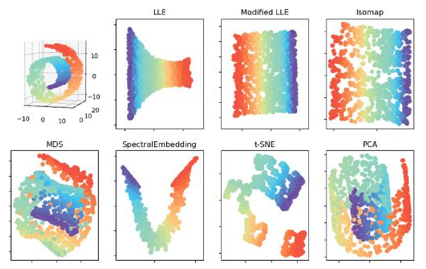
(Rabadan-Blumberg 2020)

Local Linear Embedding (LLE)

LLE is a variation of isomap manifold learning that is “locally linear.” It does not attempt to preserve the metric globally. The algorithm is a little more efficient than isomap as well.

LLE Procedure

Suppose we are given the data set $\{{\mathbf{x}}_1,\dots ,{\mathbf{x}}_m\}\subset {\mathbb{R}}^n$, the target dimension $k\in \mathbb{N}$ and a “neighborhood size” $K$.

(1) Find minimizer weights:

For each ${\mathbf{x}}_i$, find weights $w_{ij}$ that minimize the error:

$$\mathcal{E}=\sum _i{\left({\mathbf{x}}_i-\sum _j{w}_{ij}{\mathbf{x}}_j\right)}^2$$

subject to the constraints:

$$\{\begin{array}{rl}{w}_{ij}& =0\text{ if }{\mathbf{x}}_i,{\mathbf{x}}_j\text{ are NOT }K\text{-neighbors}\\ & \\ \sum _j{w}_{ij}& =1\end{array}$$

The weights determine approximations of a point using the plane that best fits its neighbors. If the manifold is actually linear around a point, the error at that point will be zero.

(2) Use minimizer weights to recover points:

Find points $\{y_1,\dots ,y_m\}\subset {\mathbb{R}}^k$ that minimize the error:

$$\mathcal{E}=\sum _i{\left(y_i-\sum _j{w}_{ij}{y}_j\right)}^2$$

The new embedding is $\theta :x_i⟼y_i$.

Locality

The Isomap and LLE algorithms are local, meaning that the output $\theta (x)$ is determined by the data around $x$. Data points far from $x$ have no effect on $\theta (x)$.