W04 Notes

Bernoulli process

01 Theory - Bernoulli, binomial, geometric, Pascal, uniform

Theory 1 - Bernoulli, binomial, geometric, Pascal, uniform

In a Bernoulli process, an experiment with binary outcomes is repeated; for example flipping a coin repeatedly. Several discrete random variables may be defined in the context of some Bernoulli process.

Notice that the sample space of a Bernoulli process is infinite: an outcome is any sequence of trial outcomes, e.g. $HTHHTTHHHTTTHHHHTTTT\cdots$

Bernoulli variable

A random variable $X_i$ is a Bernoulli indicator, written $X_i\sim \mathrm{Ber}(p)$, when $X_i$ indicates whether a success event, having probability $p$, took place in trial number $i$ of a Bernoulli process.

Bernoulli PMF:

$$P_{X_i}(k)=\{\begin{array}{ll}p& k=1\\ q& k=0\\ 0& \text{else}\end{array}$$

Here $q=1-p$.

An RV that always gives either $0$ or $1$ for every outcome is called an indicator variable.

Binomial variable

A random variable $S$ is binomial, written $S\sim \text{Bin}(n,p)$, when $S$ counts the number of successes in a Bernoulli process, each having probability $p$, over a specified number $n$ of trials.

Binomial PMF:

$$P_S(k)=\left(\genfrac{}{}{0ex}{}{n}{k}\right)p^k(1-p{)}^{n-k}\text{for }k=0,1,2,\dots ,n$$

• For example, if $S\sim \mathrm{Bin}(10,0.2)$, then $P_S(5)$ gives the odds that success happens exactly 5 times over 10 trials, with probability $0.2$ of success for each trial.
• In terms of the Bernoulli indicators, we have: $S=X_1+X_2+\cdots +X_n$
• If $A$ is the success event, then $p=P[A]$ is the success probability, and $q=1-p$ is the failure probability.

---

Geometric variable

A random variable $N$ is geometric, written $N\sim \mathrm{Geom}(p)$, when $N$ counts the discrete wait time in a Bernoulli process until the first success takes place, given that success has probability $p$ in each trial.

Geometric PMF:

$$P_N(k)=q^{k-1}p\text{for }k=1,2,3,\dots$$

Here $q=1-p$.

• For example, if $N\sim \mathrm{Geom}(30\%)$, then $P_N(7)$ gives the probability of getting: failure on the first $6$ trials AND success on the $7^{\text{th}}$ trial.

---

Pascal variable

A random variable $L$ is Pascal, written $L\sim \mathrm{Pasc}(\ell ,p)$, when $L$ counts the discrete wait time in a Bernoulli process until success happens $\ell$ times, given that success has probability $p$ in each trial.

Pascal PMF:

$$P_L(k)=\left(\genfrac{}{}{0ex}{}{k-1}{\ell -1}\right)(1-p{)}^{k-\ell }{p}^{\ell }\text{for }k=\ell ,\ell +1,\ell +2,\dots$$

• For example, if $L\sim \mathrm{Pasc}(3,0.25)$, then $P_L(8)$ gives the probability of getting: the $3^{\text{rd}}$ success on (precisely) the $8^{\text{th}}$ trial.
• Interpret the formula: $\#$ ways to arrange $2$ successes among $7$ ‘prior’ trials, times the probability of exactly $3$ successes and $5$ failures in one specific sequence.
• The Pascal distribution is also called the negative binomial distribution, e.g. $L\sim \mathrm{Negbin}(\ell ,p)$.

---

Uniform variable

A discrete random variable $X$ is uniform on a finite set $A\subset S$, written $X\sim \mathrm{Unif}(\mathrm{A})$, when the probability is a fixed constant for outcomes in $A$ and zero for outcomes outside $A$.

Discrete uniform PMF:

$$P_X(k)=\{\begin{array}{ll}\frac{1}{|A|}& \text{when }k\in A\\ 0& \text{when }k\notin A\end{array}$$

Continuous uniform PDF:

$$f_X(x)=\{\begin{array}{ll}\frac{1}{P[A]}& \text{when }x\in A\\ 0& \text{when }x\notin A\end{array}$$

Link to original

02 Illustration

Example - Roll die until

Roll die until

Roll a fair die repeatedly. Find the probabilities that:

(a) At most 2 threes occur in the first 5 rolls.

(b) There is no three in the first 4 rolls, using a geometric variable.

Solution

(a)

(1) Label variables and events:

Use a variable $S\sim \mathrm{Bin}(5,1/6)$ to count the number of threes among the first six rolls.

Seek $P[S\le 2]$ as the answer.

---

(2) Calculations:

Divide into exclusive events:

$$\begin{array}{c}P[S\le 2]\gg \gg P_S(0)+P_S(1)+P_S(2)\\ \\ \gg \gg \left(\genfrac{}{}{0ex}{}{5}{0}\right){\left(\frac{1}{6}\right)}^0{\left(\frac{5}{6}\right)}^5+\left(\genfrac{}{}{0ex}{}{5}{1}\right){\left(\frac{1}{6}\right)}^1{\left(\frac{5}{6}\right)}^4+\left(\genfrac{}{}{0ex}{}{5}{2}\right){\left(\frac{1}{6}\right)}^2{\left(\frac{5}{6}\right)}^3\\ \\ \gg \gg \frac{625}{648}\gg \gg \approx 0.965\end{array}$$

---

(b)

(1) Label variables and events:

Use a variable $N\sim \mathrm{Geom}(1/6)$ to give the roll number of the first time a three is rolled.

Seek $P[N>4]$ as the answer.

---

(2) Compute:

Sum the PMF formula for $\mathrm{Geom}(1/6)$:

$$P[N>4]\gg \gg \sum _{k=5}^{\infty }{\left(\frac{5}{6}\right)}^{k-1}\left(\frac{1}{6}\right)$$

---

(3) Recall geometric series formula:

For any geometric series:

$$a+ar+a{r}^2+a{r}^3+\cdots =\frac{a}{1-r}$$

Therefore:

$$P[N>4]=\sum _{k=5}^{\infty }{\left(\frac{5}{6}\right)}^{k-1}\left(\frac{1}{6}\right)\gg \gg {\left(\frac{5}{6}\right)}^4$$ Link to original

Example - Cubs winning the World Series

Cubs winning the World Series

Suppose the Cubs are playing the Yankees for the World Series. The first team to 4 wins in 7 games wins the series. What is the probability that the Cubs win the series?

Assume that for any given game the probability of the Cubs winning is $p=45\%$ and losing is $q=55\%$.

Solution

Method (a): We solve the problem using a binomial distribution.

(1) Label variables and events:

Use a variable $X\sim \mathrm{Bin}(7,p)$. This $X$ counts the number of wins over 7 games. Thus, for example, $P_X(4)$ is the probability that the Cubs win exactly 4 games over 7 played.

Seek $P_X(4)+P_X(5)+P_X(6)+P_X(7)$ as the answer.

---

(2) Calculate using binomial PMF:

$$P_X(k)=\left(\genfrac{}{}{0ex}{}{7}{k}\right)p^k{q}^{7-k}$$

Insert data:

$$\begin{array}{c}{P}_X(4)+\cdots +P_X(7)\\ \\ \gg \gg \left(\genfrac{}{}{0ex}{}{7}{4}\right)p^4{q}^3+\left(\genfrac{}{}{0ex}{}{7}{5}\right)p^5{q}^2+\left(\genfrac{}{}{0ex}{}{7}{6}\right)p^6{q}^1+\left(\genfrac{}{}{0ex}{}{7}{7}\right)p^7{q}^0\end{array}$$

Compute:

$$\begin{array}{c}\gg \gg \frac{7\cdot 6\cdot 5}{3\cdot 2}{p}^4{q}^3+\frac{7\cdot 6}{2}{p}^5{q}^2+\frac{7}{1}{p}^6{q}^1+1\cdot p^7{q}^0\\ \\ \gg \gg p^4(35q^3+21p^1{q}^2+7p^{2}q+p^3)\end{array}$$

Convert $q\gg (1-p)$:

$$\begin{array}{c}\gg \gg p^4(35(1-p{)}^3+21p(1-p{)}^2+7p^2(1-p)+p^3)\\ \\ \gg \gg 35p^4-84p^5+70p^6-20p^7\gg \gg \approx 0.39\end{array}$$

---

Method (b): We solve the problem using a Pascal distribution instead.

(1) Label variables and events:

Use a variable $Y\sim \mathrm{Pasc}(4,p)$. This $Y$ measures the discrete wait time until the $4^{\text{th}}$ win. Thus, for example, $P_Y(k)$ is the probability that the Cubs win their $4^{\text{th}}$ game on game number $k$.

Seek $P_Y(4)+P_Y(5)+P_Y(6)+P_Y(7)$ as the answer.

---

(2) Calculate using Pascal PMF:

$$P_Y(k)=\left(\genfrac{}{}{0ex}{}{k-1}{3}\right)p^4{q}^{k-4}$$

Insert data:

$$\begin{array}{c}{P}_Y(4)+\cdots +P_Y(7)\\ \\ \gg \gg \left(\genfrac{}{}{0ex}{}{3}{3}\right)p^4{q}^0+\left(\genfrac{}{}{0ex}{}{4}{3}\right)p^4{q}^1+\left(\genfrac{}{}{0ex}{}{5}{3}\right)p^4{q}^2+\left(\genfrac{}{}{0ex}{}{6}{3}\right)p^4{q}^3\end{array}$$

Compute:

$$\begin{array}{c}\gg \gg 1\cdot p^4+\frac{4}{1}\cdot p^4{q}^1+\frac{5\cdot 4}{2}{p}^4{q}^2+\frac{6\cdot 5\cdot 4}{3\cdot 2}{p}^4{q}^3\\ \\ \gg \gg p^4(1+4q+10q^2+20q^3)\end{array}$$

Convert $q\gg (1-p)$:

$$\begin{array}{c}\gg \gg p^4(1+4(1-p)+10(1-p{)}^2+20(1-p{)}^3)\\ \\ \gg \gg 35p^4-84p^5+70p^6-20p^7\gg \gg \approx 0.39\end{array}$$

---

Notice: The calculation seems very different than method (a), right up to the end!

Link to original

Expectation and variance

03 Theory - Expectation and variance

Theory 1

Expected value

The expected value $E[X]$ of random variable $X$ is the weighted average of the values of $X$, weighted by the probability of those values.

Discrete formula using PMF:

$$E[X]=\sum _{k}k\cdot P_X(k)$$

Continuous formula using PDF:

$$E[X]={\int }_{-\infty }^{+\infty }x\cdot f_X(x)dx$$

Notes:

• Expected value is sometimes called expectation, or even just mean, although the latter is best reserved for statistics.
• The Greek letter $\mu$ is also used in contexts where ‘mean’ is used.

---

Let $X$ be a random variable, and write $E[X]=\mu$.

Variance

The variance $\mathrm{Var}[X]$ measures the average squared deviation of $X$ from $\mu$. It estimates how concentrated $X$ is around $\mu$.

• Defining formula:

$$\mathrm{Var}[X]=E[(X-\mu {)}^2]$$

• Shorter formula:

$$\mathrm{Var}[X]=E[X^2]-E[X{]}^2$$

Calculating variance

• Discrete formula using PMF:

$$\mathrm{Var}[X]=\sum _k(k-\mu {)}^2{P}_X(k)$$

• Continuous formula using PDF:

$$\mathrm{Var}[X]={\int }_{-\infty }^{+\infty }(x-\mu {)}^2{f}_X(x)dx$$

Standard deviation

The quantity ${\sigma }_X=\sqrt{\mathrm{Var}[X]}$ is called the standard deviation of $X$.

Link to original

04 Illustration

Example - Tokens in bins

Gambling game - tokens in bins

Consider a game like this: a coin is flipped; if $H$ then draw a token from Bin 1, if $T$ then from Bin 2.

• Bin 1 contents: 1 token $1,000, and 9 tokens $1
• Bin 2 contents: 5 tokens $50, and 5 tokens $1

It costs $50 to enter the game. Should you play it? (A lot of times?) How much would you pay to play?

Solution

(1) Setup:

Let $X$ be a random variable measuring your winnings in the game.

The possible values of $X$ are 1, 50, and 1000.

---

(2) Find the PDF of $X$:

For $k=1$ have $P_X(1)\gg \gg \frac{1}{2}\cdot \frac{9}{10}+\frac{1}{2}\cdot \frac{5}{10}\gg \gg \frac{7}{10}$

For $k=50$ have $P_X(50)\gg \gg \frac{1}{2}\cdot \frac{5}{10}\gg \gg \frac{1}{4}$

For $k=1000$ have $P_X(1000)\gg \gg \frac{1}{2}\cdot \frac{1}{10}\gg \gg \frac{1}{20}$

These add to 1, and $P_X(x)=0$ for all other $x$.

---

(3) Find $E[X]$ using the discrete formula:

$$\begin{array}{c}E[X]=\sum _{k}k\cdot P_X(k)\gg \gg 1\cdot P_X(1)+50\cdot P_X(50)+1000\cdot P_X(1000)\\ \\ \gg \gg 1\cdot \frac{7}{10}+50\cdot \frac{1}{4}+1000\cdot \frac{1}{20}\gg \gg \approx 63.2\end{array}$$

Since $63.2>50$, if you play it a lot at $50 you will generally make money.

---

Challenge Q:
If you start with $200 and keep playing to infinity, how likely is it that you go broke?

Link to original

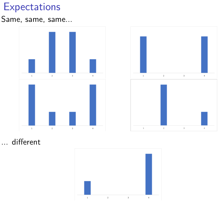
Example - Expected value: rolling dice

Expected value: rolling dice

Let $X$ be a random variable counting the number of dots given by rolling a single die.

Then:

$$E[X]\gg \gg 1\cdot \frac{1}{6}+2\cdot \frac{1}{6}+\cdots +6\cdot \frac{1}{6}\gg \gg \frac{7}{2}$$

Let $S$ be an RV that counts the dots on a roll of two dice.

The PMF of $S$:

Then:

$$E[S]\gg \gg 2\cdot \frac{1}{36}+3\cdot \frac{2}{36}+4\cdot \frac{3}{36}+\cdots +12\cdot \frac{1}{36}\gg \gg 7$$

Notice that $\frac{7}{2}+\frac{7}{2}=7$.

In general, $E[X+Y]=E[X]+E[Y]$.

Let $X$ be a green die and $Y$ a red die.

From the earlier calculation, $E[X]=\frac{7}{2}$ and $E[Y]=\frac{7}{2}$.

Since $S=X+Y$, we derive $E[S]=7$ by simple addition!

Link to original

Example - Expected value by finding new PMF

Expected value by finding new PMF

Let $X$ have distribution given by this PMF:

Find $E[|X-2|]$.

Solution

(1) Compute the PMF of $|X-2|$:

PMF arranged by possible value:

$$\begin{array}{rl}P[|X-2|=0]& \gg \gg P[X=2]=\frac{1}{14}\\ P[|X-2|=1]& \gg \gg P[X=1]+P[X=3]=\frac{1}{7}+\frac{3}{14}=\frac{5}{14}\\ P[|X-2|=2]& \gg \gg P[X=4]=\frac{2}{7}\\ P[|X-2|=3]& \gg \gg P[X=5]=\frac{2}{7}\\ P[|X-2|=k]& \gg \gg 0\text{for}k\ne 0,1,2,3.\end{array}$$

---

(2) Calculate the expectation:

Using formula for discrete PMF:

$$E[|X-2|]\gg \gg 0\cdot \frac{1}{14}+1\cdot \frac{5}{14}+2\cdot \frac{2}{7}+3\cdot \frac{2}{7}\gg \gg \frac{25}{14}$$ Link to original

Exercise - Variance using simplified formula

Variance for composite using PMF and simpler formula

Suppose $X$ has this PMF:

$k:$	1	2	3
$P_X(k):$	$1/7$	$2/7$	$4/7$

Find $\mathrm{Var}\left[\frac{1}{1+X}\right]$ using the formula $\mathrm{Var}[Y]=E[Y^2]-E[Y{]}^2$ with $Y=\frac{1}{1+X}$.

(Hint: you should find $E[Y]=\frac{13}{42}$ and $E[Y^2]=\frac{13}{126}$ along the way.)

Link to original