Chapter 05 - Manifolds and Morse Theory

Manifolds

Theory - Topological and smooth manifolds

Topological and smooth manifolds

Topological manifold

A (second-countable, Hausdorff) topological space $X$ is an $n$-dimensional (topological) manifold if every point $p\in X$ has an open neighborhood $U$ which is homeomorphic to ${\mathbb{R}}^n$.

$$\text{“ the local topology of an n-manifold is that of Rn ”}$$

Notes:

• An equivalent definition is that every $p$ has open neighborhood $U$ homeomorphic to the open ball ${\mathbb{B}}_1(0)\in {\mathbb{R}}^n$, since of course ${\mathbb{B}}_1(0)$ is itself homeomorphic to ${\mathbb{R}}^n$.
• It is a theorem that every $n$-manifold can be embedded in some Euclidean space ${\mathbb{R}}^N$, so an equivalent definition states adds the hypothesis that $X\subset {\mathbb{R}}^N$ for some $N$.

---

To define smooth manifolds, we must first define differentiable and smooth maps.

Regular points

Suppose $p\in V\subset {\mathbb{R}}^n$ with $V$ open. Let $(x_1,\dots ,x_n)$ give coordinates on ${\mathbb{R}}^n$.

Suppose $f:V\to {\mathbb{R}}^d$ is a function given in coordinates by $f(x_1,\dots ,x_n)=(f_1,\dots ,f_d)$.

The differential matrix of $f$ at $p=(x_1,\dots ,x_n)$ is the Jacobi matrix:

$$[d_{p}f]=\left(\begin{array}{ccc}\frac{\partial f_1}{\partial x_1}(p)& \cdots & \frac{\partial f_1}{\partial x_n}(p)\\ ⋮& \ddots & ⋮\\ \frac{\partial f_d}{\partial x_1}(p)& \cdots & \frac{\partial f_d}{\partial x_n}(p)\end{array}\right)$$

The point $p$ is regular for $f$ when $[df]$ has rank $n$.
(No point can be regular when $d<n$.)

Smooth manifold in ${\mathbb{R}}^d$

A subspace $M\subset {\mathbb{R}}^d$ is a smooth $n$-manifold if every $p\in M$ has an open neighborhood in $M$ (open in the subspace topology) that is the image of a smooth injective function $\phi :U\to {\mathbb{R}}^d$, whose domain is an open set $U\subset {\mathbb{R}}^n$, and whose differential $[d\phi ]$ has maximal rank everywhere on $U$.

Each such function is called a parametrization or a coordinate chart for $M$, and the image of a parametrization is a coordinate patch on $M$.

---

A parametrized surface is a bijective and infinitely differentiable (smooth) injective map:

$$\phi :U\to {\mathbb{R}}^3$$

where the parameter domain $U$ is an open subset of ${\mathbb{R}}^2$. Every parametrized surface defines a $2$-manifold in ${\mathbb{R}}^3$.

Using coordinates $(x,y)$ on ${\mathbb{R}}^2$ and $({\phi }_1,{\phi }_2,{\phi }_3)$ for the images of $\phi$ in ${\mathbb{R}}^3$, we have for the differential matrix:

$$[d_{(x,y)}\phi ]=\left(\begin{array}{cc}\frac{\partial {\phi }_1}{\partial x}& \frac{\partial {\phi }_1}{\partial y}\\ \frac{\partial {\phi }_2}{\partial x}& \frac{\partial {\phi }_2}{\partial y}\\ \frac{\partial {\phi }_3}{\partial x}& \frac{\partial {\phi }_3}{\partial y}\end{array}\right)$$

The maximum rank of $[d\phi ]$ is $2$, and $\mathrm{Rank}[d\phi ]=2$ occurs when any of these equivalent conditions are satisfied:

• The columns of $[d\phi ]$ are linearly independent (for two columns: not collinear vectors)
• There are two linearly independent rows in $[d\phi ]$
• There is a $2\times 2$ submatrix of $[d\phi ]$ with nonzero determinant

If the matrix $[d\phi ]$ is considered as a linear map $[d\phi ]:{\mathbb{R}}^2\to {\mathbb{R}}^3$, then the image of $[d\phi ]$ at $p=(x,y)$ is a plane through the origin which is parallel to the tangent plane to the surface at $\phi (x,y)$.

The condition $\mathrm{Rank}[d\phi ]=2$ ensures that small movements in the parameter space, $dx$ and $dy$, can generate two dimensions of movement on the surface. In turn this ensures that locally around $\phi (x,y)$ the surface is homeomorphic to an open disk in ${\mathbb{R}}^2$, and moreover that such a homeomorphism can be constructed as projection to the tangent plane at $\phi (x,y)$ composed with a linear map.

Link to original

Illustration

Wild topological manifolds

Wild topological manifolds

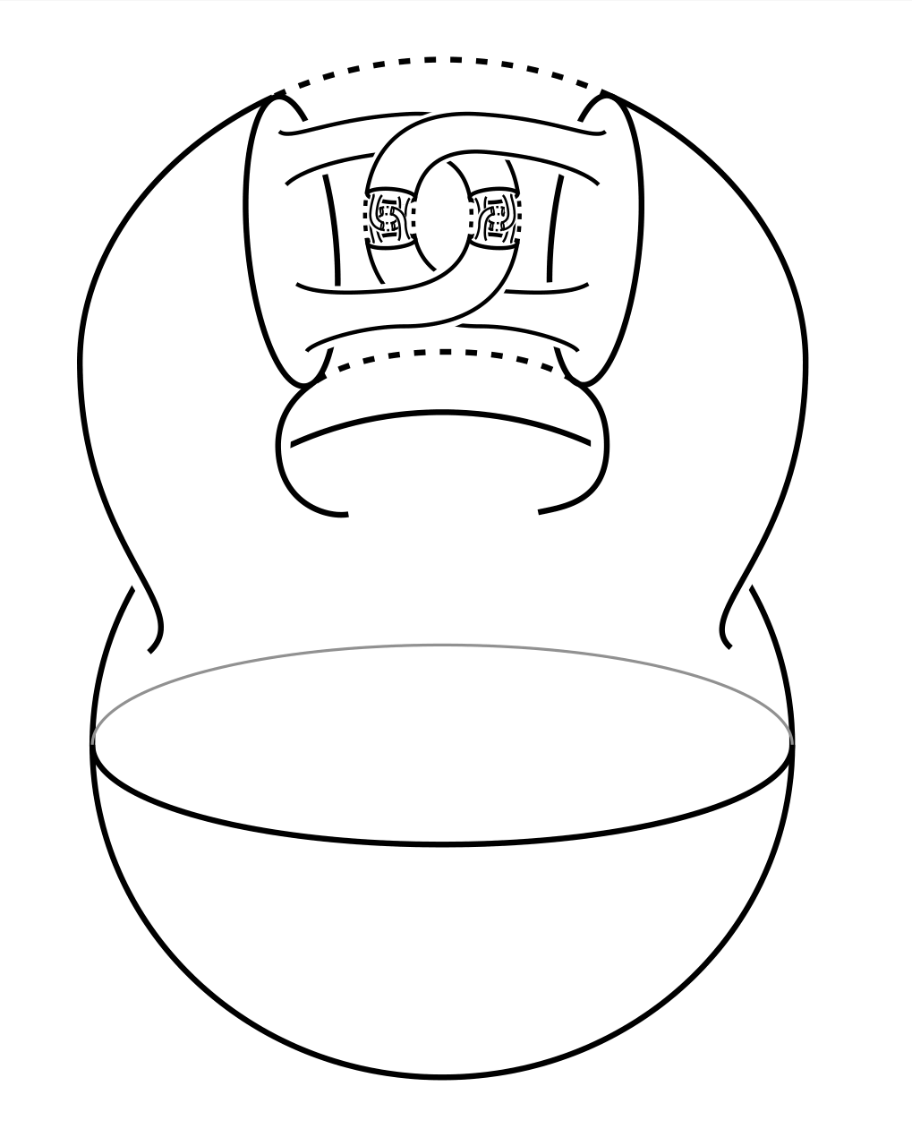
Topological spaces can be stranger than one imagines on the basis of simple examples. Here is Alexander’s Horned Sphere (https://en.wikipedia.org/wiki/Alexander_horned_sphere; explanatory essay):

The horned sphere $S$ is a subset of ${\mathbb{R}}^3$ homeomorphic to ${\mathbb{S}}^2$. The outside ${\mathbb{R}}^3-S$ contains non-collapsible loops (so it is not simply connected), which is unlike the standard inclusion of ${\mathbb{S}}^2$ in ${\mathbb{R}}^3$.

The map $f:{\mathbb{S}}^2\hookrightarrow {\mathbb{R}}^3$ with $f({\mathbb{S}}^2)=S$ is an embedding of topological spaces and thus topological manifolds. (It is continuous, injective, and induces a homeomorphism onto the image which is endowed with the subspace topology; so the image is homeomorphic to ${\mathbb{S}}^2$ as a topological manifold.)

The map $f$ is not an embedding of differentiable, smooth, or piecewise linear manifolds.

Link to original

Parametrized paraboloid

Parametrized paraboloid

Let $\phi :{\mathbb{R}}^2\to {\mathbb{R}}^3$ by $\phi :(x,y)\mapsto \left(x,y,x^2+y^2\right)$.

Then $[d\phi ]$ is given by:

$$[d_{(x,y)}\phi ]=\left(\begin{array}{cc}1& 0\\ 0& 1\\ 2x& 2y\end{array}\right)$$

Notice that the determinant of the upper $2\times 2$ square is nonzero.

Link to original

Singular curve

Singular curve

Consider $\phi :\mathbb{R}\to {\mathbb{R}}^2$ given by $\phi (t)=(t^2,t^3)$:

Then: $[d_t\phi ]=\left[\begin{array}{c}2t\\ 3t^2\end{array}\right]$ and $[d_0\phi ]=\left[\begin{array}{c}0\\ 0\end{array}\right]$.

Link to original

Parametrized 2-sphere

Parametrized 2-sphere

Spherical coordinates define a parametrization of the 2-sphere:

$$f(\theta ,\phi )=\left(\sin \phi \cos \theta ,\sin \phi \sin \theta ,\cos \phi \right)$$

The differential:

$$[d_{(x,y)}\phi ]=\left(\begin{array}{cc}\cos \phi \cos \theta & -\sin \phi \sin \theta \\ \cos \phi \sin \theta & \sin \phi \cos \theta \\ -\sin \phi & 0\end{array}\right)$$

Notice that poles of the sphere correspond to points with $\phi =n\pi$, and there the right column is all zeros. So poles are not regular points of $\phi$. One can check that every other point is regular by computing the cross product of the column vectors.

Also, at the poles the function is not injective.

Therefore one must restrict the domain, for example to $\phi \in (-\pi ,\pi )$ and $\theta \in (0,2\pi )$, to get a true parametrization. Unfortunately this does not cover the entire sphere; indeed it is impossible to cover the sphere with a single parametrization.

Link to original

Parametrized 2-torus in R4

Parametrized 2-torus in ${\mathbb{R}}^4$

The 2-torus can be parametrized in ${\mathbb{R}}^4$ very easily:

$$f(\phi ,\theta )=\left(\cos \phi ,\sin \phi ,\cos \theta ,\sin \theta \right)\phi ,\theta \in (0,2\pi )$$

This parametrization is regular everywhere, but the domain cannot be extended to cover the entire torus without becoming non-injective (and no longer a homeomorphism onto its image), for topological reasons. The torus cannot be covered by a single parametrization.

Link to original

Manifolds cont’d

Theory - Local coordinates

Local coordinates

Smooth map

A map $\phi :U\to V$ for open sets $U\subset {\mathbb{R}}^n$ and $V\subset {\mathbb{R}}^d$ is smooth when all partial derivatives of all orders exist and are continuous.

A map $\phi$ is a diffeomorphism when it is a homeomorphism and both $\phi$ and ${\phi }^{-1}$ are smooth.

Suppose we have $\phi :U\to {\mathbb{R}}^d$ a smooth map for $U\subset {\mathbb{R}}^n$ open, $n\le d$, and we know $\phi$ is injective and $[d_p\phi ]$ has maximal rank for all $p\in U$.

Then the Inverse Function Theorem from multivariable real analysis implies that ${\phi }^{-1}$ is also a smooth map from $\phi (U)$ to $U$.

Therefore the parametrizations (charts) of a smooth manifold are diffeomorphisms.

Local coordinates

Given a coordinate chart $\phi$ for a smooth manifold $M$, the coordinates of the images of the inverse ${\phi }^{-1}$ provide local coordinates on $M$.

Link to original

Illustration

Smooth injection phi but inverse of phi not smooth

Smooth injection $\phi$ but ${\phi }^{-1}$ not smooth

Let $f:\mathbb{R}\to \mathbb{R}$ given by $f(x)=x^3$. Clearly $f$ is infinitely differentiable and injective.

Notice $f^{\prime }(0)=0$. So the differential does not have maximal rank at $x=0$.

The inverse function $\sqrt[3]{x}$ is not smooth, indeed it is not differentiable at $x=0$.

Link to original

Circle requires two charts

Circle requires two charts

Show that it is not possible to cover the unit circle ${\mathbb{S}}^1\subset {\mathbb{R}}^2$ with a single coordinate chart.

Solution

Suppose the contrary, that $\phi :U\to {\mathbb{R}}^2$ for $U\subset \mathbb{R}$ is a coordinate chart covering ${\mathbb{S}}^1$.

(We assume this means $U$ is connected.)

---

Let $p\in {\mathbb{S}}^1$ be some point. Set $A={\mathbb{S}}^1-\{p\}$.

• Then $A$ is connected.
• Therefore ${\phi }^{-1}(A)$ is connected since ${\phi }^{-1}$ is a homeomorphism.

---

Set $q={\phi }^{-1}(p)$.

• Then ${\phi }^{-1}(A)=U-\{q\}$.
• $U-\{q\}$ is disconnected: the open sets $U\cap \{x<q\}$ and $U\cap \{x>q\}$ separate $U-\{q\}$.
• So ${\phi }^{-1}(A)$ is disconnected and connected, a contradiction.

Link to original

Morse theory

Theory - Gradient, critical points; Hessian, non-degenerate points

Gradient, critical points; Hessian, non-degenerate points

Suppose we are given a smooth function $f:{\mathbb{R}}^d\to \mathbb{R}$.

The differential matrix of $f$ in this case is (the transpose of) the gradient of $f$:

$$\nabla f(p)=[d_{p}f{]}^{\mathsf{T}}={\left(\begin{array}{c}\frac{\partial f}{\partial x_1}(p),\frac{\partial f}{\partial x_2}(p),\dots ,\frac{\partial f}{\partial x_d}(p)\end{array}\right)}^{\mathsf{T}}$$

By the definition of regular point, a point $p\in {\mathbb{R}}^d$ is regular for $f$ when the gradient vector is not $\vec{0}$, i.e. when $\frac{\partial f}{\partial x_i}(p)\ne 0$ for some coordinate $x_i$. The point $p$ is called critical when it is not regular.

(Note: $f$ is smooth by hypothesis, so the components of $\nabla f$ are everywhere defined, and so critical points are points where $\nabla f=\vec{0}$.)

---

The differential $[d_{p}f]$ of a smooth function $f:{\mathbb{R}}^d\to \mathbb{R}$ is itself a smooth function ${\mathbb{R}}^d\to {\mathbb{R}}^d$. We may thus take the differential of the differential, and we obtain the Hessian matrix of second partial derivatives:

$$[H_p(f)]=\left(\begin{array}{cccc}\frac{{\partial }^{2}f}{\partial x_1^2}& \frac{{\partial }^{2}f}{\partial x_1\partial x_2}& \cdots & \frac{{\partial }^{2}f}{\partial x_1\partial x_n}\\ ⋮& ⋮& \ddots & ⋮\\ \frac{{\partial }^{2}f}{\partial x_n\partial x_1}& \frac{{\partial }^{2}f}{\partial x_n\partial x_2}& \cdots & \frac{{\partial }^{2}f}{\partial x_n^2}\end{array}\right)$$

The Hessian matrix is always a symmetric square matrix because $\frac{{\partial }^{2}f}{\partial x_i\partial x_j}=\frac{{\partial }^{2}f}{\partial x_j\partial x_i}$. This implies that all eigenvalues are real numbers (a case of the Spectral Theorem).

Non-degenerate critical point

A critical point $p$ for a function $f:{\mathbb{R}}^d\to \mathbb{R}$ is non-degenerate when $[H_p(f)]$ is a non-singular matrix.

Equivalently, when:

• $\det [H_p(f)]\ne 0$
• All eigenvalues of $[H_{p}f]$ are nonzero

Index of a critical point

Given a non-degenerate critical point $p$, the index of $p$ is the number of negative eigenvalues of $[H_p(f)]$.

Isolated critical point

A critical point $p$ for a function $f:{\mathbb{R}}^d\to \mathbb{R}$ is isolated when an open neighborhood of $p\in {\mathbb{R}}^d$ can be found such that $p$ is the only critical point of $f$ in this neighborhood.

Link to original

Illustration

Same critical point, different index

Same critical point, different index

Consider these functions from ${\mathbb{R}}^2$ to $\mathbb{R}$:

$$\begin{array}{rl}f(x,y)& =x^2+y^2\\ g(x,y)& =x^2-y^2\\ h(x,y)& =-x^2-y^2\end{array}$$

The point $p=(0,0)$ is the only critical point for each of these functions.

The Hessian matrices at $p$ are:

$$[H_p(f)]=\left(\begin{array}{cc}2& 0\\ 0& 2\end{array}\right)[H_p(g)]=\left(\begin{array}{cc}2& 0\\ 0& -2\end{array}\right)[H_p(h)]=\left(\begin{array}{cc}-2& 0\\ 0& -2\end{array}\right)$$

So $p$ has index $0$ for $f$, index $1$ for $g$, and index $2$ for $h$.

Link to original

Theory - Morse functions on manifolds

Morse functions on manifolds

Morse theory is about the use of a function $f:M\to \mathbb{R}$ to study the topology of the manifold $M$ in terms of the critical points of $f$. One sets up a function $f$ that has nondegenerate critical points with distinct critical values, called a Morse function. To make sense of this setup we need first to define smooth functions $f:M\to \mathbb{R}$.

Smooth function on a manifold

A function $f:M\to \mathbb{R}$ on a smooth manifold $M\subset {\mathbb{R}}^d$ is smooth if it is the restriction of a smooth function $\tilde{f}:U\to \mathbb{R}$ where $U$ is an open set in ${\mathbb{R}}^d$ with $M\subset U\subset {\mathbb{R}}^d$.

This means: $f=\tilde{f}{|}_M$ and $\tilde{f}$ has continuous partial derivatives of all orders.

---

Recall local coordinates:
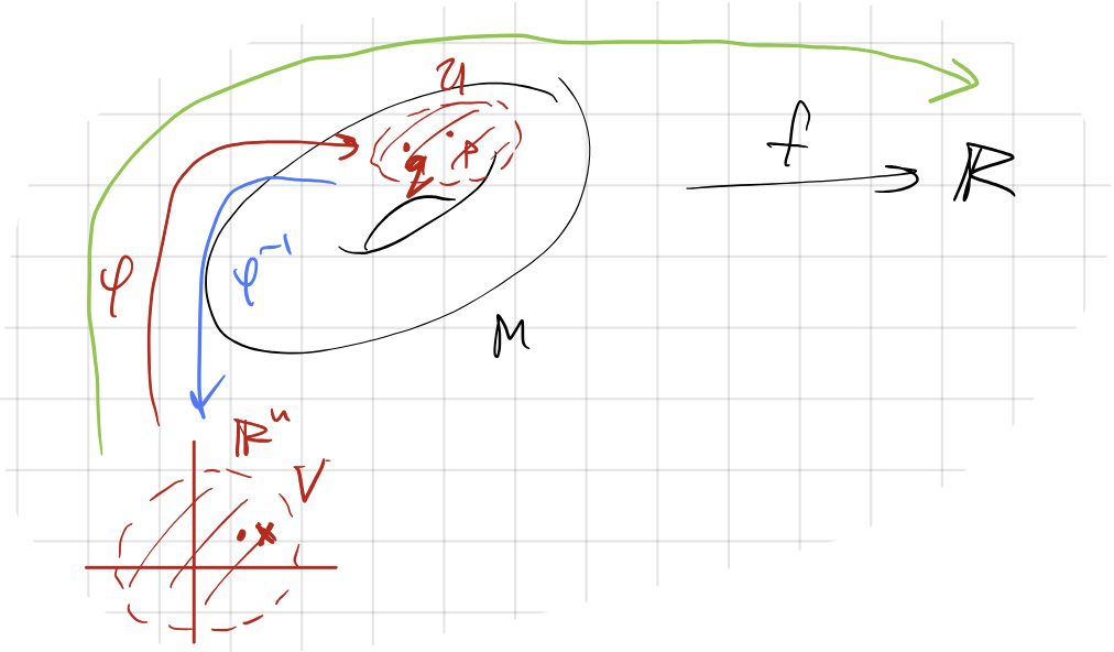
For any $p\in M$ there is a set $V\ni p$ open in ${\mathbb{R}}^n$ and $U$ open in $M$ with

$$\phi :V\to U$$

a parametrization (diffeomorphism to its image). The ${\mathbb{R}}^n$-coordinates of images of the inverse ${\phi }^{-1}$ give local coordinates on $U$.

Critical and non-degenerate, from a manifold

Let $f:M\to \mathbb{R}$ be a smooth function on a smooth $n$-manifold in ${\mathbb{R}}^d$, and $\phi :V\to U$ a parametrization of the open neighborhood $U$ of $p$. So $f\circ \phi :V\to \mathbb{R}$ for $V\subset {\mathbb{R}}^n$.

Choose any $q\in U$. Set $x={\phi }^{-1}(q)$.

We say $q$ or $x$ is regular when $\nabla (f\circ \phi )(x)\ne \vec{0}$ and critical when $\nabla (f\circ \phi )(x)=\vec{0}$.

We say $q$ or $x$ is non-degenerate when $[H_x(f\circ \phi )]$ is a non-singular matrix (and degenerate otherwise).

Notice that this definition of regularity appears to depend on the parametrization $\phi$. But in fact, the definition is independent of the choice of $\phi$:

Proposition - Regularity is independent of parametrization

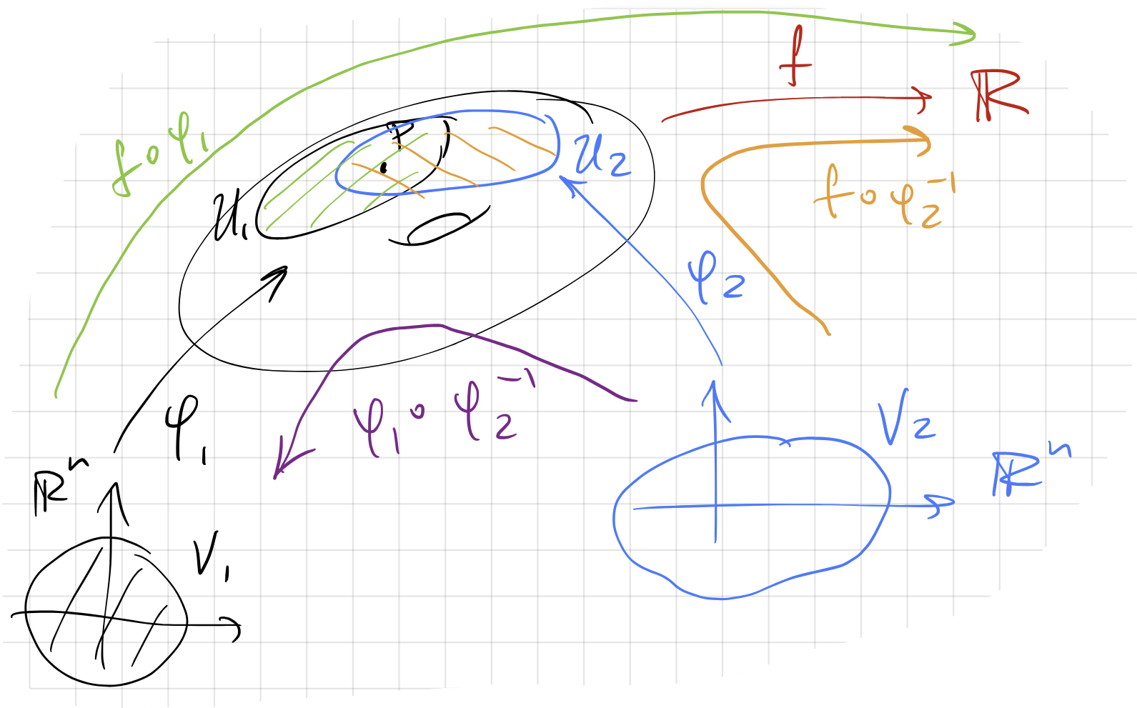
Suppose we are given two parametrizations ${\phi }_1$ and ${\phi }_2$ of a coordinate patch $U\subset M$.

Take an arbitrary $q\in U$ and assume it is regular according to ${\phi }_1$.

We show it must be regular according to ${\phi }_2$.

This will complete the proof because if it is critical according to ${\phi }_1$, and not critical according to ${\phi }_2$, then it is regular according to ${\phi }_2$, and the same argument can be run after switching ${\phi }_1\leftrightarrow {\phi }_2$.

---

Define the ‘transition map’ $\psi ={\phi }_1^{-1}\circ {\phi }_2$.

This $\psi$ is a map $V_1\to V_2$ where ${\phi }_1:V_1\to U$ and ${\phi }_2:V_2\to U$ for $V_i\subset {\mathbb{R}}^n$ open balls.

Notice that $(f\circ {\phi }_2)=(f\circ {\phi }_1)\circ \psi$.

---

Apply chain rule:

$$\nabla (f\circ {\phi }_2)=\nabla (f\circ {\phi }_1\circ \psi )=\nabla (f\circ {\phi }_1)\circ [d\psi ]$$

Here $[d\psi ]$ is the Jacobi matrix of $\psi$.

---

Argue that $[d\psi ]$ is invertible:

We have that $[d{\phi }_1]$ and $[d{\phi }_2]$ are both isomorphisms from ${\mathbb{R}}^n$ to the tangent space of $M$ at $q$.

Then $[d\psi ]$ is the composition of $[d{\phi }_2]$ with the inverse of $[d{\phi }_1]$ restricted to the tangent space of $M$ at $q$. (Prior to restriction $[d{\phi }_1]$ is not even a square matrix.)

Therefore $[d\psi ]$ is invertible.

Therefore, at any point:

$$\nabla (f\circ {\phi }_2)=0⟺\nabla (f\circ {\phi }_1\circ \psi )=0$$

So a point is regular for ${\phi }_1$ if and only if it is regular for ${\phi }_2$.

Why define regularity using parametrizations?

Since the choice of parametrization has no effect on the classification of points as regular or critical, one may wonder why the parametrization is needed at all.

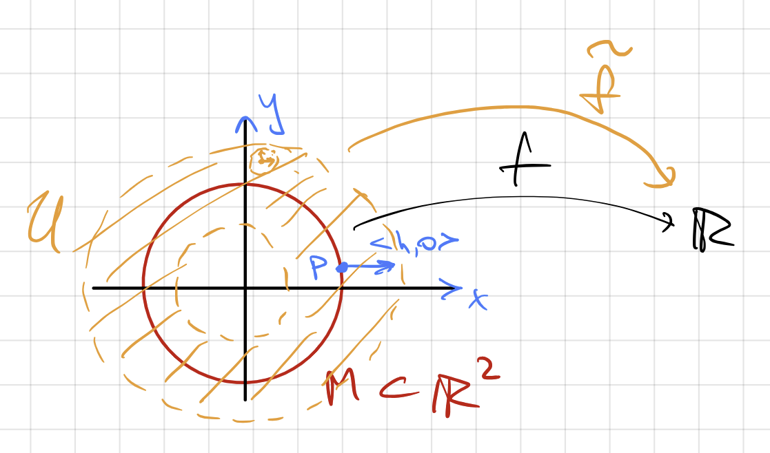
But the concept of regularity does involve the manifold’s embedding, and not just the values of $f$ in the ambient space around the manifold.

A point $q\in M$ is regular for $f$ when there is some first-order infinitesimal deviation of $q$ within $M$ which causes a first-order deviation in $f$. When $q$ is critical, the induced change in $f$ is second order at most.

For example, given a smooth function $f:{\mathbb{R}}^n\to \mathbb{R}$, a level surface $M$ is (frequently) an $(n-1)$-manifold every point of which is regular for $f:{\mathbb{R}}^n\to \mathbb{R}$, but no point of which is regular for $f{|}_M:M\to \mathbb{R}$.

Tangent space $T_{p}M$

Given a manifold $M\subset {\mathbb{R}}^d$, we define the tangent space to $M$ at $p\in M$, written $T_{p}M$, as the image of $[d_p\phi ]$ in ${\mathbb{R}}^d$ for $\phi$ any parametrization of a neighborhood of $p$.

Comparing gradient functions

Notice:

• $\nabla \tilde{f}$ is a map from ${\mathbb{R}}^d$, and has $d$ coordinates
• $\nabla (f\circ \phi )$ is a map from ${\mathbb{R}}^n$, and has $n$ coordinates, one for each dimension of $M$

In general: ${\nabla }_p(f\circ \phi )$ is the restriction of ${\nabla }_p\tilde{f}$ to $T_{p}M$ using columns of $[d\phi ]$ as a basis.

(Supposing $M\subset {\mathbb{R}}^d$ and $\tilde{f}$ an extension of $f:M\to \mathbb{R}$ to $U$ with $M\subset U\subset {\mathbb{R}}^d$.)

---

Morse Lemma

Suppose $q$ is a non-degenerate critical point of index $i$ of a smooth function $f:M\to \mathbb{R}$.

Then:

$$f\circ \phi =x_1^2+\cdots +x_{n-i}^2-x_{n-i+1}-\cdots -x_n^2$$

for some parametrization $\phi$ whose local coordinates are $x_1,\dots ,x_n$.

Morse functions

A Morse function $f:M\to \mathbb{R}$ is a smooth function from a manifold $M\subset {\mathbb{R}}^d$ to $\mathbb{R}$ which satisfies:

1. All critical points of $f$ are non-degenerate.
2. The values of $f$ at its critical points are all distinct.

Morse functions are dense

Morse functions are dense in the space of smooth functions.

There is a small perturbation of any smooth function that is a Morse function.

Link to original

Illustration

Height function

Height function

Suppose $\tilde{f}:{\mathbb{R}}^3\to \mathbb{R}$ by $\tilde{f}(x,y,z)=z$.

Then $\nabla \tilde{f}=(0,0,1)$. Since $\nabla (f\circ \phi )$ is the restriction of $\nabla \tilde{f}$ to $T_{p}M$, we see that $p$ is critical for $f$ precisely when $T_{p}M$ is normal to $(0,0,1)$.

In other words: critical points of $f$ are points where the tangent space to $M$ is a horizontal plane.

This reasoning generalizes to higher dimensions ${\mathbb{R}}^d$ where one dimension is chosen as ‘vertical’, and horizontal planes become hypersurfaces normal to the vertical unit vector.

Link to original

Theory - Morse functions and topology

Morse functions and topology

Given a Morse function $f:M\to \mathbb{R}$ for a manifold $M$, define:

• $M_C=f^{-1}(C)$ the level set at $C$
• $M_{\le C}=f^{-1}((-\infty ,C])$ the sublevel set under $C$

By continuously increasing the value of $C$ (starting at $-\infty$), we find that the topology of $M_{\le C}$ changes exactly when $C$ passes a critical point of $f$.

Sublevel set builds topology

Up to homotopy equivalence, as $C$ passes through a critical point of index $k$, the sublevel set changes by the attachment of a $k$-ball along its boundary.

For example:

• Pass a point of index $2$ $⇝$ glue on a disk, a lid opening downwards
• Pass a point of index $1$ $⇝$ glue on an arc (up to homotopy)
• Pass a point of index $0$ $⇝$ create a new disk, a basket opening upwards

Link to original

Illustration

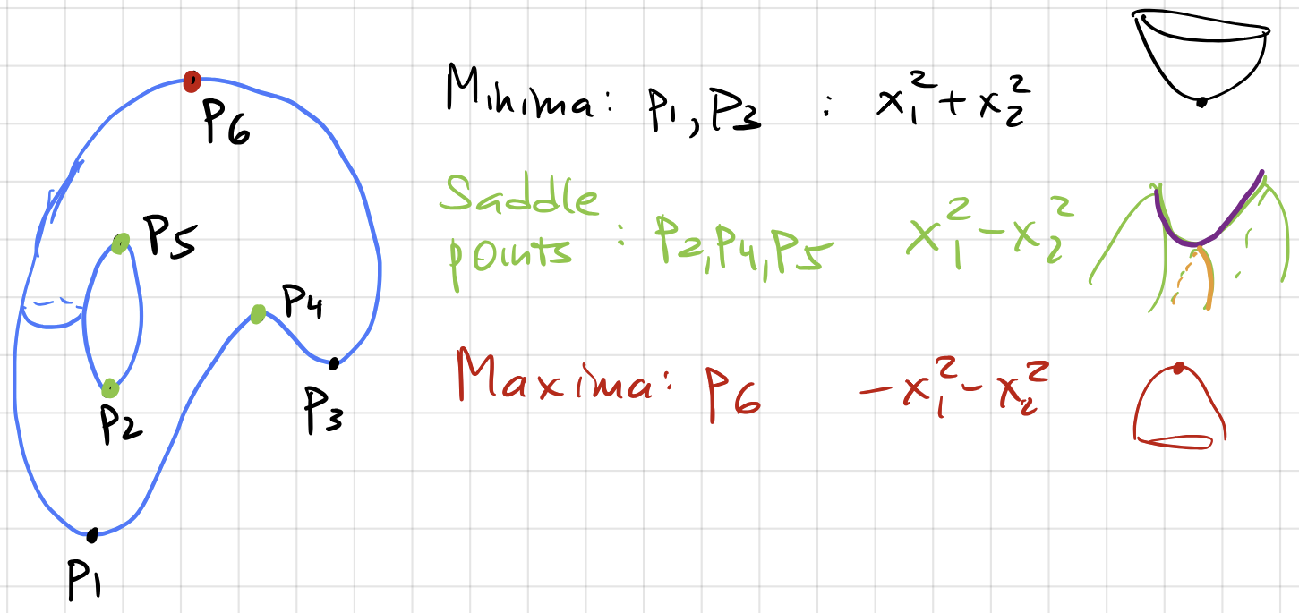
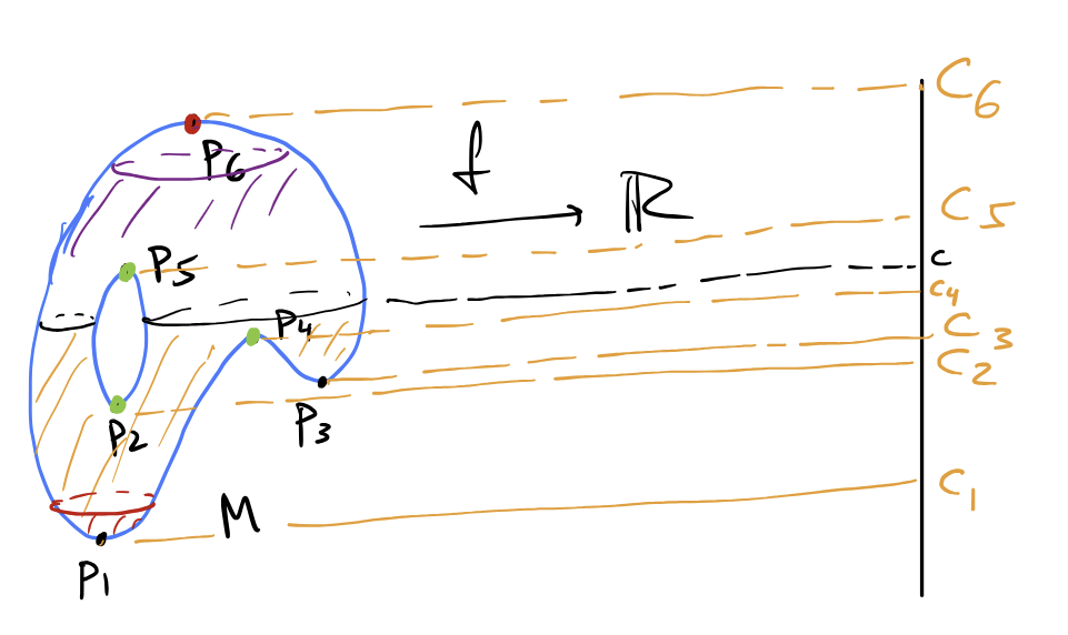
Height function on a torus

Height function on a torus

Suppose $f:{\mathbb{R}}^3\to \mathbb{R}$ is the height function $f(x,y,z)=z$, and $M$ is topologically a torus, though not geometrically.

As $C$ passes through $f(P_1)$, a small disk is created in $M_{\le C}$.

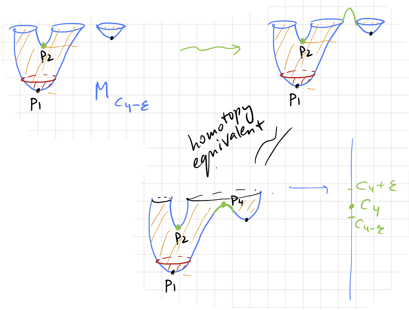
Passing through $f(P_2)$ is (up to homotopy) equivalent to adding a handle to the basket below $C_2$:

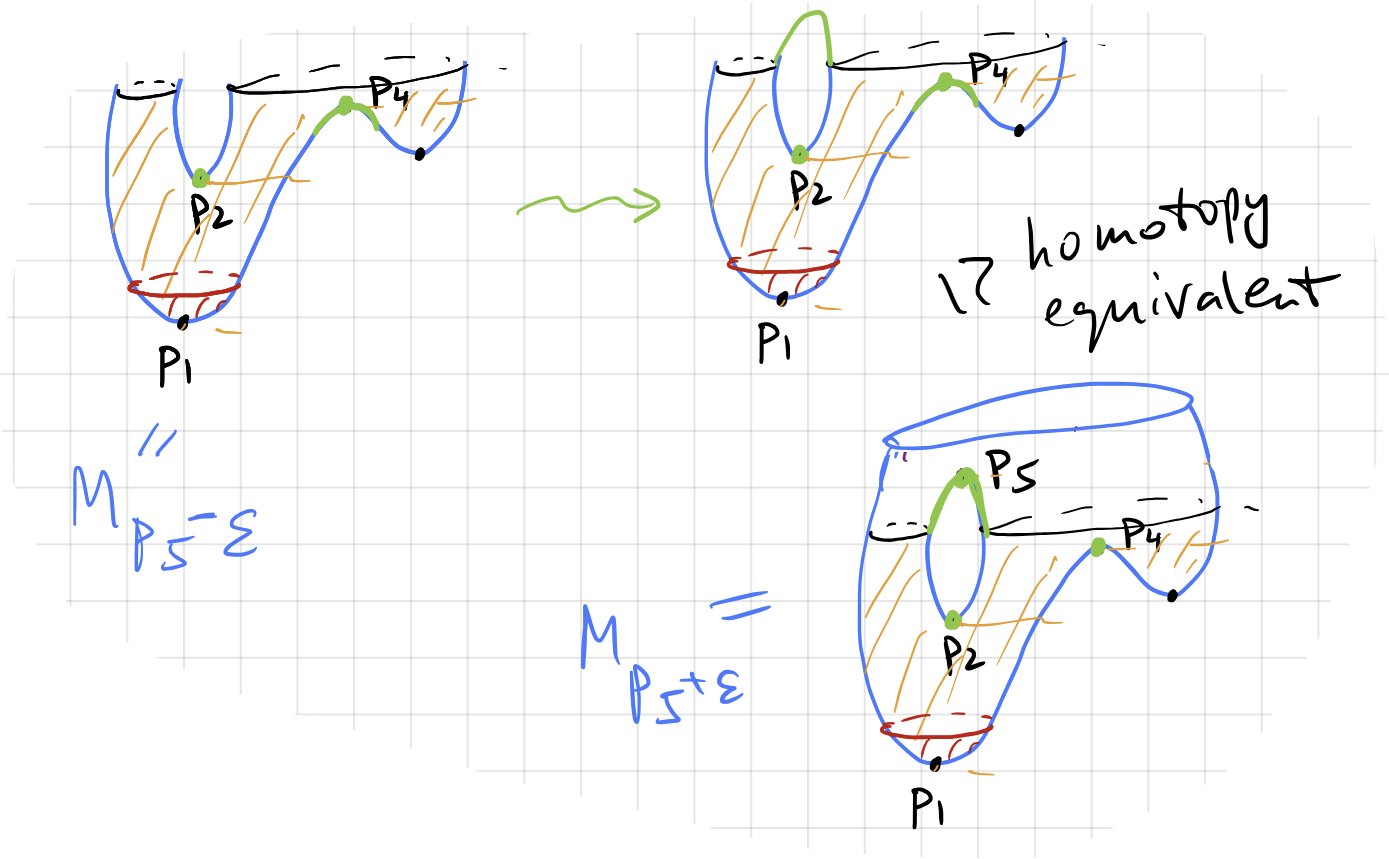
Passing through $f(P_3)$ adds a new basket, and passing through $f(P_4)$ adds a handle connecting the basket:

Passing through $f(P_5)$ adds a handle creating a loop:

Link to original