Matrices III: Inner Products
Introduction
In this section we study some interrelated concepts: orthogonal matrices, symmetric matrices, inner products, quadratic forms, and positive definite matrices.
Link to original
Orthogonal matrices
Orthogonal matrices
A matrix is called orthogonal when it satisfies .
‘Orthogonal’ ‘orthonormal’ for matrices
The term orthonormal is also used for the same class of matrices. (Warning! Not so for vectors! Orthogonal vectors are merely perpendicular, while orthonormal vectors are also unit vectors.)
Now consider the meaning of the formula . Remember the rule for matrix products (e.g. in D):
What is ? Each row of this vector is the dot product of the same row of with the vector . In turn, each row of is from a column of . Combining all these claims with the product rule, column of has rows equal to the dot products of the various columns of with the specific column of . Specifically, . In conclusion, means that
It follows that is another way of saying that and are mutually orthonormal. So, if you put an orthonormal basis into the column vectors of a matrix, the resulting matrix is orthogonal. Conversely, if a matrix is orthogonal, then its columns form an orthonormal basis. (They are orthonormal by the definition of orthogonal, and they are a basis because they are perpendicular and thus independent.)
An important fact about orthogonal matrices is that they correspond geometrically to rotations and reflections (and combinations of these actions called ‘rotoreflections’).
Orthogonal matrices preserve the dot product, preserving lengths and angles
The action of an orthogonal matrix preserves the dot product:
Link to originalWhy
To see this, recall (1) our interpretation of row vectors as matrices, and (2) the dot product with as the action of the transpose row vector acting by matrix multiplication on the left, so e.g. . Using this, we derive:
Symmetric matrices
Symmetric matrices
A symmetric matrix is a matrix that satisfies . In terms of coefficients, this means it satisfies . A symmetric matrix is symmetric about reflection in a mirror that runs down the main diagonal:
An antisymmetric matrix (also called skew-symmetric) satisfies , in other words .
Symmetric matrices do arise naturally in many applications. This can happen for a variety of reasons. One example is PCA (principal component analysis): here the matrix in question arises as a “covariance matrix,” and it is symmetric because covariance is symmetric: . Antisymmetric matrices are less common.
Symmetric matrices have some very nice properties:
Spectral theorem
Let be any symmetric matrix, so . Then:
- (a) has the max number of eigenvalues (some might be repeated, but they still exist).
- (b) All eigenvalues of are real numbers.
- (c) Eigenvectors with distinct eigenvalues are perpendicular to each other.
- (d) There is an orthonormal basis such that becomes diagonal in this basis: in other words . Notice that is an orthogonal matrix, and are eigenvectors of .
Proofs of most of these facts are just a little beyond the scope of a first applied course. Part (c) is not hard though:
Orthogonal eigenvectors of a symmetric matrix
Suppose and and . Assume, as we do for eigenvectors, that . Then consider the sequence:
Therefore, we find that . This can only happen if , which we have denied by hypothesis, or else if , which must therefore be true.
The equation is equivalent to a very nice formula for called the spectral decomposition formula:
In this formula, the are the orthogonal basis given by the spectral theorem (remember they are also eigenvectors), and the are the corresponding eigenvalues.
SVD prelude
The spectral decomposition is an instance of the singular value decomposition (SVD) which works for general matrices. Stay tuned for more in the section on the SVD!
A great thing about this formula is that each is actually a projection matrix onto :
Why? Of course . Since are unit vectors, we have . This is the same thing, just written with a different order for the scalar factor (result of the dot product).
Link to original[Optional] Explaining the spectral decomposition formula
The spectral decomposition formula itself comes from writing out the matrices in :
Quadratic forms and symmetric matrices
Quadratic forms and symmetric matrices
A quadratic form is a function from vectors to scalars that can be written as a polynomial with all terms having degree . For example:
In short, a quadratic form is just a polynomial in several variables that is homogeneous of degree . (‘Homogeneous’ just means that all terms have the same degree.) The difference between quadratic forms and quadratic polynomials is that the latter could also have terms of degree zero and degree one.
Link to originalApplications of quadratic forms
The simplest possible quadratic form is the sum of squares: . Notice that this form gives the square distance from to . One strong application of linear algebra is the ability to extremize quadratric forms. For example, in Linear Least Squares, we extremize the distance from a point to a certain span. We will shortly see how to represent this distance as a quadratic form. In Weighted LLS, we minimize the distance with inequal weights applied to each term, such as in . This kind of weighting is useful when some data is more reliable than other data, so it should be given more weight.
Question
[Removed!]
Quadratic forms and symmetric matrices (part 2)
Key fact:
Link to originalMatrix of a quadratic form
Every quadratic form can be represented uniquely by a symmetric matrix, meaning there is some symmetric such that .
So there is a perfect correspondence between quadratic forms and symmetric matrices.
Example
Quadratic form
Link to originalQuadratic form
Question
01
Link to originalMatrix of a quadratic form
What is the matrix such that is the quadratic form ?
Quadratic forms and symmetric matrices (part 3)
A quadratic form can always be converted into a new quadratic form that has no cross terms by a suitable linear change of variables. If the original variables are the components of , then a linear change of variables would be a vector defined by for some change of basis transfer matrix .
Principal axes theorem: eliminating cross terms
Given a quadratic form defined by the symmetric matrix , suppose . Set , so also . Then has no cross terms in the variables.
Link to originalDerivation
First plug in the new variables and manipulate:
This last expression has no cross terms:
Example
Eliminating cross terms
Link to originalEliminating cross terms
Problem: Eliminate the cross terms in the quadratic form .
Solution: First compute the matrix of . By reading off the components (dividing in half the cross term), we see
Now we must write for an orthogonal matrix. We find the eigenvalues and then seek eigenvectors that are orthonormal. Observe that , so the eigenvalues are .
Then we have:
so gives the relation satisfied by the rows of an eigenvector. Choose and then normalize this to the unit vector .
Then we also have:
so and we choose as an eigenvector, and normalize to the unit vector . Notice that .
Now we set and and write our expression for :
In terms of the variables, we have . The formulas relating the variables to each other are given by interpreting as the change of variable transfer matrix:
Exercise
01
Link to originalEliminating cross terms.
Repeat the example to eliminate cross terms for the quadratic form .
Constrained optimization, min-max principle
Constrained optimization, min-max principle
One simple yet important application of elimination of cross terms is constrained optimization. The goal of constrained optimization is to find the extreme values of a quadratic form where is constrained to be a unit vector, so . Geometrically, this means: find the direction of fastest increase or direction of fastest decrease of , and find the rate of increase / decrease in those directions.
If we have written so as to eliminate cross terms:
then the max / min of occurs for where is the max / min coefficient.
If is not written without cross terms, then we can first eliminate cross terms completely, and find the max / min among the set of . This will give the max / min value, and the input where this occurs in terms of the variables at . The change of variables must be made in reverse to find the corresponding input values where the max / min occurs. If the eigenvector corresponding to has already been found, its components are by definition the components of that we seek.
Link to original
Example
Optimizing the quadratic form from the eliminating cross terms example
Link to originalOptimizing
In the Example of the previous section on eliminating cross terms, we obtained the formula for in terms of the variables . We can see directly from this formula that the min eigenvalue is and the max eigenvalue is .
The min of occurs when . In other words it is at the first eigenvector . In terms of the variables, this occurs at and , the components of in the standard basis.
The max of occurs when . In other words at , which corresponds to and .
Exercise
02
Link to originalOptimizing
Repeat the example on this quadratic form, using your work in Exercise 12-01, to find the min and max of for a unit vector, and find the unit vectors that produce these extreme values.
Constrained optimization, min-max principle (part 2)
However, it is not necessary to find all of the . These are the eigenvalues / eigenvectors, and there are some methods of computing eigenvalues that locate the largest / smallest values by a numerical procedure that does not waste time finding the other values. The power method is an example of such a method. (Read more about the power method online, if you like.)
Link to originalMin-max principle and Rayleigh quotient
A closely related topic is the min-max principle for finding eigenvalues using the Rayleigh quotient. Given any symmetric matrix , its Rayleigh quotient is:
Notice that the value of is the same as the value of the quadratic form generated by , evaluated at the unit vector given by first normalizing the input . Therefore, maximizing over all possible is the same as maximizing the quadratic form of over all possible unit vectors.
The min-max principle is simply this: the min / max eigenvalues of are the min / max values of , and these occur when is an eigenvector for that eigenvalue. The use of this principle is to find min / max eigenvalues / eigenvectors of a symmetric by extremizing with numerical methods (like the power method and its variants).
The min-max principle and Rayleigh quotient is essentially just a notation and terminology for the process of normalizing and plugging it into the quadratic form arising from the symmetric matrix .
Positive definite symmetric matrices
Positive definite symmetric matrices
- A positive definite matrix is by definition a symmetric matrix all of whose eigenvalues are greater than zero.
- A negative definite matrix is by definition a symmetric matrix all of whose eigenvalues are less than zero.
- An indefinite matrix is by definition a symmetric matrix whose eigenvalues have mixed signs.
For example, in terms of spectral decompositions, we have:
Since the spectral decomposition reveals the quadratic form in the new variables, where , but these input variables cover the same set of possibilities, we also know:
Link to originalQuadratic forms definiteness
- When is positive definite, then its form is always positive for .
- When is negative definite, then its form is always negative for .
Inner products and symmetric matrices
Inner products and symmetric matrices
An inner product is a function sending two vector inputs to one scalar output:
which is linear in both inputs considered separately.
Rules of inner products:
- Symmetry.
- Respects sums (also in using symmetry).
- Respects scalars (also in using symmetry).
- for all , and only occurs when .
We are very familiar with the dot product, which is a valid inner product:
Using the linearity of matrix actions, we can create many candidate inner products by first acting by a symmetric matrix and then taking the usual dot product:
This definition of is automatically symmetric (i.e. it satisfies the symmetry rule) because is symmetric:
If you take any inner product given by a symmetric matrix, and plug the input into both slots, you get a quadratic form:
The last property of inner products (namely that etc.) means that a quadratic form created in this way by setting is always a positive definite quadratic form.
Conversely, any inner product is given by some positive definite symmetric matrix. To find the matrix corresponding to an inner product, simply set . This works because gives the column vector of , and then gives the row entry of this column, which is therefore the row and column entry of . By linearity, is then determined on every other pair of vectors by this data.
Link to original
Addendum: determinants and eigenvectors
Addendum - determinants and eigenvectors
The determinant of a matrix is given by the formula:
The determinant of a matrix is given by the formula:
Higher determinants
You may notice a pattern here that hold true in general and allows calculation of determinants: traverse any row or column, using these entries as weights (with alternating signs), writing a weighted sum of the smaller determinants of the minor matrices (which are given by deleting the row and column in which the given entry in our traversal process lives). This process therefore reduces an determinant to a linear combination of determinants, and the reduction can be iterated until the case is reached.
The characteristic polynomial of a matrix is defined as the determinant in which is considered an indefinite variable.
For example: if then and (using the determinant formula) we have:
Key fact for finding eigenvalues
The eigenvalues of a matrix are the roots of its characteristic polynomial .
In the previous example, therefore, are the eigenvalues.
Once the eigenvalues are found by solving for , the solutions can be plugged back in for in the equation , and then we can try to find the eigenvectors by solving this equation. For the case, you can solve it using the fact that one row is a multiple of the other. In and higher, you may need to perform row reduction on (with ) in order to find solutions .
Notice that if is an eigenvector, then is also an eigenvector for any scalar . So really we are studying eigenlines, namely the spans of eigenvectors. The relation of proportionality between and gives the direction of this line.
For in the previous example, solving would mean solving . Therefore and thus , so an eigenvector is given by and a line of eigenvectors is given by the span for all . For we find , and solving this we find and therefore is an eigenvector, as is everything in the span .
Link to original
Matrices IV: Spectrum
Eigenvectors, eigenvalues: Part II
Example
Finding eigenvectors and eigenvalues
Link to originalFinding eigenvectors and eigenvalues
Problem: Find the eigenvectors and their eigenvalues for the matrix .
Solution: First find the eigenvalues:The roots are . (The rational roots theorem leads to the guess , and then you can divide the cubic polynomial by to obtain a quadratic one, which is easily factored.)
Now we seek eigenvectors by solving for each root. When :
To solve for , row reduce to obtain a matrix in RREF:
So we know and is free. Plugging these in we have , and we choose obtaining for an eigenvector.
Next for we have:
To solve for , row reduce to obtain a matrix in RREF:
So we know and . Plugging these in we have , and we choose obtaining .
Finally for we have:
To solve for , row reduce to obtain a matrix in RREF:
So we know and . Plugging these in we have , and we choose obtaining .
Example
Changing to eigenbasis yields diagonal matrix
Link to originalChanging to eigenbasis yields diagonal matrix
Notice that in the previous example has three eigenvectors, and that they are independent. Therefore they constitute a basis of ; let’s call this basis . Putting these basis vectors as the columns of a matrix, we create the change of basis transfer matrix from to the standard basis :
So .
Now consider that these are eigenvectors of with eigenvalues :
If we write in the basis using the transfer matrix , we have:
In other words, the matrix of is a diagonal matrix when written in the basis of its own eigenvectors.
Eigenvectors, eigenvalues - Part II
The example above illustrates a general fact: if a matrix has enough independent eigenvectors to form a basis of the vector space on which acts, then if you write in the basis of these eigenvectors, it will have a diagonal form.
In other words, the eigenbasis of is a natural basis for . It is a basis in which the action of is extremely simple: it is given by scaling the basis vectors by the respective eigenvalue numbers.
Sometimes a matrix has not enough independent eigenvectors. Here is an illustration:
Link to original
Example
Matrix with too few eigenvectors
Link to originalMatrix with too few eigenvectors
The matrix has . Therefore it has a “double” eigenvalue . To find the eigenvectors:
The matrix is already in RREF. So the equation says that is free and . Therefore we have the eigenvector .
However, no more eigenvectors are available (other than scalar multiples of this one, which would not be independent of this one). Therefore it is impossible to find a basis of eigenvectors, and it is thus impossible to convert to diagonal form by a change of basis.
Eigenvectors, eigenvalues - Part II (part 2)
Sometimes a real matrix has complex eigenvalues and eigenvectors. Here is an illustration:
Link to original
Example
Matrix with complex eigenvalues and eigenvectors
Link to originalMatrix with complex eigenvalues and eigenvectors
The matrix has so its eigenvalues are . To find the eigenvectors:
Row reduce the matrix :
This is now in RREF, so we see that and is free, so we get the eigenvector .
Following the same procedure for , we find the eigenvector .
Eigenvectors, eigenvalues - Part II (part 3)
It is important to be aware of these two situations. For the sake of exams, you should memorize one example of each type. (You can use the two above.)
Link to original
Question
01
Link to originalDouble eigenvalues does not imply insufficient eigenvectors
What are the eigenvalues and eigenvectors of ? Are there enough to form a basis of ?
Question
02
Link to originalEnough eigenvectors?
Does the matrix have enough eigenvectors to form a basis? If not, how many does it have?
Eigenvectors, eigenvalues - Part II (part 4)
Link to originalSpectral Theorem: symmetric matrices have good eigen theory
A key point of the Spectral Theorem is that symmetric matrices never encounter the phenomena illustrated in the two examples above. Eigenvalues are always real numbers, and there are always enough eigenvectors to form a basis.
Eigenvectors vs. singular vectors
Eigenvectors vs. singular vectors
It is helpful to think about the concept of an eigenvector as consisting of two aspects:
- (1) Matrix acting by scaling
- (2) Fixed lines of matrix action
Aspect (1) allows easy computation and geometric understanding of the matrix action. It also allows us to focus on vectors that are more important (those having a larger scale factor). If we have a basis of such vectors, the matrix will have a simple diagonal form when written in this basis.
Aspect (2) goes much further, even though it essentially includes aspect (1). A fixed line (eigenline) is the span of any eigenvector. Such lines are mapped to themselves by the matrix action. This aspect describes eigenvector spans as analogues of fixed points of a function. The concept of fixed points and fixed lines (‘fixity’ in general) only applies when the function or matrix keeps vectors in the same space, i.e. has the same codomain as domain.
Eigenvectors
There are various contexts where a matrix does act on vectors in a single space. Aspect (2) is very useful in these contexts. For example, a differential operator, which produces a system of first-order linear differential equations, involves a matrix for a vector space of functions . For another example, the moment of inertia matrix describing angular moment of D bodies in physics. Or the many operators of quantum mechanics.One of the biggest advantages of aspect (2) is that it is compatible with iteration.
If is a linear transformation (i.e. a matrix) having the same codomain as domain, we can define iterates etc. as matrix powers. These powers allow one to apply functions to matrices: if is a power series, we can define by the power series . (Bracketing any problems with convergence.) An extremely important series is , since the function solves the linear ODE system .
It is hard to compute , or more generally , by direct multiplication and limits of partial sums. On the other hand, it is easy to compute when is a diagonal matrix, just as it is easy to compute when is an eigenvector of . (Namely, the latter is .) For example, in the case we have .
Even when is not diagonal, if an eigenbasis matrix can be found, then the powers of are still easy to calculate, because (e.g. in D):
Similarly we have:
The critical piece of the calculation above is the cancellation occurring in the calculation for . This cancellation shows that matrix multiplication and change of basis can be performed in either order. That in turn means we can first change basis to an eigenbasis (if it exists) and then perform multiplication with the diagonal matrices where it is easy, and only afterwards change back to the standard basis.
Singular vectors
The concept of singular vector is designed to make use of aspect (1) of eigenvectors without aspect (2). Because they do not include aspect (2), singular vectors of are not eigenvectors of except in special cases. They do not determine fixed lines of the action.Unlike eigenvectors and eigenvalues, singular vectors and singular values are (best) defined in the context of a collection of vectors giving the singular value decomposition (SVD). So, a singular vector is one of the vectors in the SVD.
Link to original
Defining the singular value decomposition
Defining the singular value decomposition
Suppose is a matrix providing a linear transformation between different vector spaces.
SVD features
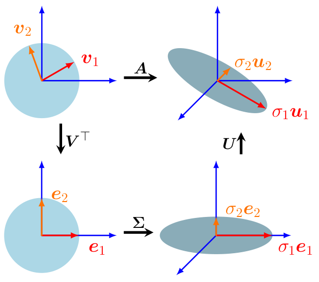
A singular value decomposition of is given by: where:
- is an orthogonal matrix giving a rotation/reflection combo for (input)
- is an orthogonal matrix giving a rotation/reflection combo for (output)
- has non-negative entries on the main diagonal (possibly zeros!) and zeros elsewhere. (Here .) It is not square if . It could look like these, for example:
The orthonormal basis vectors are called right singular vectors.
The orthonormal basis vectors are called left singular vectors.
The values are the lengths of the images, namely .(Remember: “Right Input, Left Output.”)
An alternate way to write the SVD uses scalar projections attached to the vectors :
Each term takes an input vector, dots it with , then applies this value to scaled by . With this formula, we can compute for any input using dot products:
By plugging in , we verify that and , etc. up to . (For , we have .)
Singular vectors vs. eigenvectors
The rule looks analogous to the rule for eigenvectors.
But it’s actually very different! Notice that and are not even vectors in the same space!
The rule does not by itself determine any special property of or . (Take any unit vector , apply , then define and .)
The significance of the rule manifests when it holds simultaneously on all vector pairs in orthonormal bases and .
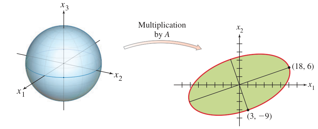
Still, the SVD says that after rotating / reflecting the basis of and the basis of by suitable orthogonal matrices (not necessarily the same on each), the action of can be represented as simple scalings by .
We may think of as a special basis for the input space vis-à-vis the matrix , and as a corresponding basis for the output space . Then acts by pairing the vector to and stretching it by .
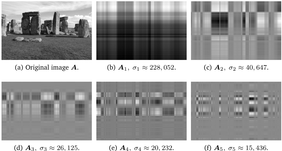
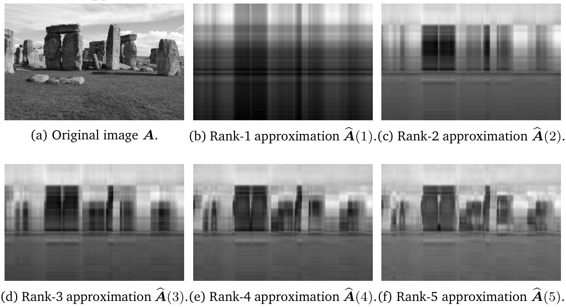
Partial matrices for .Link to original
Partial sum matrices for .
Computing the singular value decomposition
Computing the singular value decomposition
In practice, on a computer, the SVD is calculated using numerical procedures that are akin to those used to find approximations to eigenvectors. We do not address those kinds of procedures in this course.
Still, it is possible to specify and calculate SVD elements by hand for a matrix by making use of the fact that is always a symmetric matrix and the Spectral Theorem can be applied to it. This method also shows that the SVD always exists, since the symmetric always has real eigenvalues and enough eigenvectors by the Spectral Theorem, even when does not. Let us see how this works.
First observe that , so is always symmetric. Also notice that , so the input and output spaces of this matrix are the same.
Link to originalSVD elements
- orthonormal eigenbasis of .
As guaranteed by the Spectral Theorem, so here is in the notation of that theorem.- defined for .
If , then .- The equation for defines unit vectors for those with .
- Gram-Schmidt provides additional vectors when .
Example
Computing SVD by hand
Link to originalComputing SVD by hand
Problem: Find an SVD for the matrix .
Solution: First calculate that and this matrix has and eigenvalues. Therefore we set and . By solving we obtain an eigenvector which we renormalize to the unit vector . By solving we obtain an eigenvector which we renormalize to the unit vector . We now have and :
Set
and we notice that . Now we need unit vectors orthogonal to each other and to . We first calculate a span of the kernel of the matrix , and then perform Gram-Schmidt to orthogonalize it. For the kernel:
and therefore so we can set free and solve for , thereby obtaining generators for the kernel:
Now we already have by our method of defining . So it just remains to do the last step of Gram-Schmidt. We calculate that
Then
We have finished, and the SVD is given by:
Exercise
01
Link to originalComputing SVD by hand
Find an SVD for the matrix .
Exercise
02
Link to originalComputing SVD by hand
Find an SVD for the matrix .
Computing the singular value decomposition (part 2)
Explaining the SVD elements
First, why is an orthogonal matrix?
Answer: Since is an orthonormal basis, the matrix is orthogonal.
Second, why is an orthogonal matrix?
Answer: Consider the calculation:Notes: The first line is the dot product using ‘inner product’ notation. The second line is the transpose rule. The fourth line is the definition of as eigenvector of . The last line is the property that are orthonormal vectors.
From this calculation it follows that are orthogonal vectors (at least when they aren’t zero). Since are the same vectors renormalized as unit vectors, we know are orthonormal (at least when ). In the case of , the alternate definition of using Gram-Schmidt implies that all are orthonormal.
Third, why is ?
Answer: According to the calculation above, . But by definition.Fourth, why is , with these definitions of ?
Answer: To verify the equality , it is sufficient to verify that the matrices on both sides have the same action on a basis of . (If that is true, then by linearity the matrices have the same action on any vector, and therefore they are the same matrices.)Therefore, it is sufficient to verify the equality of actions on the basis . Since this basis is orthonormal, we see that is the vector with in the row and zeros elsewhere. Then is the column of , which has in the row and zeros elsewhere. Finally is the row of (which is ) scaled by . Therefore , and this is equal to . All these statements are valid for . For , both sides send to .
Link to originalBackwards: Going from SVD to eigenvectors-eigenvalues of
Addendum. If we already have an SVD given by , with on the diagonal of , then must be the eigenvectors of , and are the corresponding eigenvalues.
Proof: Observe that
where is the square diagonal matrix with diagonal entries given by . Applying the matrix to returns , which verifies the claim. (Again both matrices send to for .)