Chapter 14 - Space Curves

Parametric space curves: differentiation

Introduction

A vector-valued parametric curve in ${\mathbb{R}}^3$ may be given in terms of component functions by $\mathbf{r}(t)=(x(t),y(t),z(t))$. When the component functions are differentiable, then $\mathbf{r}(t)$ is also said to be differentiable, and the derivative function is ${\mathbf{r}}^{\prime }(t)=(x^{\prime }(t),y^{\prime }(t),z^{\prime }(t))$. Applying the same logic repeatedly, one obtains higher derivatives ${\mathbf{r}}^{(n)}(t)=(x^{(n)},y^{(n)},z^{(n)})$.

Link to original

Example

Derivative of vector function, constant basis

Derivative of vector function, constant basis

Consider $\mathbf{r}(t)=\ln (t){\mathbf{e}}_{\mathbf{i}}+t{\mathbf{e}}_{\mathbf{j}}+t^3{\mathbf{e}}_{\mathbf{k}}$. Find ${\mathbf{r}}^{\prime }(t)$ and ${\mathbf{r}}^{\prime \prime }(t)$.

Solution: Differentiation is given componentwise, so we can treat the basis vectors as constants and differentiate their coefficients: ${\mathbf{r}}^{\prime }(t)=\frac{1}{t}{\mathbf{e}}_{\mathbf{i}}+{\mathbf{e}}_{\mathbf{j}}+3t^2{\mathbf{e}}_{\mathbf{k}}$ and ${\mathbf{r}}^{\prime \prime }(t)=-\frac{1}{t^2}{\mathbf{e}}_{\mathbf{i}}+6t{\mathbf{e}}_{\mathbf{k}}$.

Link to original

Derivative rules for parametric space curves

Derivative rules for parametric space curves

Given $\mathbf{r}(t),{\mathbf{r}}_1(t),{\mathbf{r}}_2(t)$ vector functions, and $c$ a scalar, and $f(t)$ a scalar function (all differentiable), then the standard derivative rules for algebraic compositions of functions determine rules applying to vector operations: e

• Sums: $({\mathbf{r}}_1(t)+{\mathbf{r}}_2(t){)}^{\prime }={\mathbf{r}}_1^{\prime }(t)+{\mathbf{r}}_2^{\prime }(t)$
• Constants: $(c\mathbf{r}(t){)}^{\prime }=c{\mathbf{r}}^{\prime }(t)$
• Scalar products: $(f(t)\mathbf{r}(t){)}^{\prime }=f(t){\mathbf{r}}^{\prime }(t)+f^{\prime }(t)\mathbf{r}(t)$
• Chain rule: $\frac{d}{dt}\mathbf{r}(g(t))=g^{\prime }(t){\mathbf{r}}^{\prime }(g(t))$

Moreover, by considering the component formulas for vector products, one finds derivative rules for vector products analogous to the rule for a scalar product:

• Dot product rule: $({\mathbf{r}}_1(t)\cdot {\mathbf{r}}_2(t){)}^{\prime }={\mathbf{r}}_1^{\prime }(t)\cdot {\mathbf{r}}_2(t)+{\mathbf{r}}_1(t)\cdot {\mathbf{r}}_2^{\prime }(t)$
• Cross product rule: $({\mathbf{r}}_1(t)\times {\mathbf{r}}_2(t){)}^{\prime }={\mathbf{r}}_1^{\prime }(t)\times {\mathbf{r}}_2(t)+{\mathbf{r}}_1(t)\times {\mathbf{r}}_2^{\prime }(t)$

Link to original

Exercise

01

Parametric curve: derivative rules for vector products

Use the algebraic properties of dot and cross product to prove the derivative product rules without using the component descriptions of those products. (Imitate the proof of the standard product rule.)

Link to original

Derivative rules for parametric space curves (part 2)

Constant norm vector functions
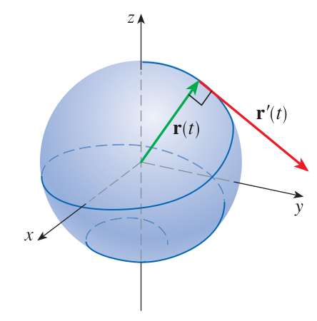
When a vector-valued parametric function has constant norm $|\mathbf{u}(t)|=c$, the vector is necessarily perpendicular to its own derivative:

$$0=\frac{d}{dt}(c^2)=\frac{d}{dt}(\mathbf{u}(t)\cdot \mathbf{u}(t))=2\mathbf{u}(t)\cdot {\mathbf{u}}^{\prime }(t).$$

This fact is often applied to the case of a unit vector. Intuitively, a unit vector gives a direction as a point on the unit sphere. An infinitesimal change of this direction will lie in the tangent plane to the sphere, which is perpendicular to the sphere, and thus perpendicular to the original vector.

Link to original

Tangent and normal vectors

Tangent and normal vectors

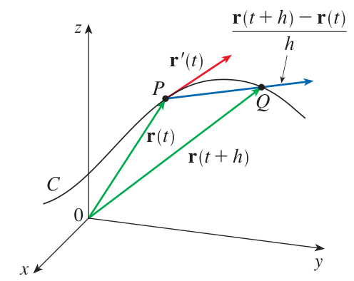
The tangent vector ${\mathbf{r}}^{\prime }(t)$ of a parametric curve is just the derivative of $\mathbf{r}(t)$ as a vector-valued parametric function. It is tangent to the curve:

When the curve is non-stationary, i.e. ${\mathbf{r}}^{\prime }(t)\ne 0$, then its tangent vector determines a unit tangent vector which is typically written $\mathbf{T}(t):=\frac{1}{|{\mathbf{r}}^{\prime }(t)|}{\mathbf{r}}^{\prime }(t)$. This vector represents the direction of travel of a particle traversing the curve.

When the component functions are twice differentiable, the unit tangent has a derivative ${\mathbf{T}}^{\prime }(t)$. Where the curve is non-straight, i.e. ${\mathbf{T}}^{\prime }(t)\ne 0$, then ${\mathbf{T}}^{\prime }(t)$ determines a unit normal vector $\mathbf{N}(t):=\frac{1}{|{\mathbf{T}}^{\prime }(t)|}{\mathbf{T}}^{\prime }(t)$, also called the principal normal vector.

$\mathbf{T}$ and $\mathbf{N}$ are perpendicular
Since $\mathbf{T}(t)$ has a constant norm of one, we know that $\mathbf{T}(t)\perp \mathbf{N}(t)$ at all times.

Link to original

Exercise

02

$\mathbf{T}$ and $\mathbf{N}$ for a circle

Compute $T$ and $N$ for the circle in the $yz$-plane given parametrically by $(0,R\cos (\theta ),R\sin (\theta ))$.

Link to original

Distance traveled, speed

Distance traveled, speed

To improve the expression of various formulas, we use the notation:

$$\mathbf{v}(t):={\mathbf{r}}^{\prime }(t).$$

The distance traveled function is given for a parametric curve in ${\mathbb{R}}^3$ by:

$$\begin{array}{rl}s(t)& ={\int }_a^t|{\mathbf{r}}^{\prime }(u)|du\\ & ={\int }_a^{t}v(u)du\\ & ={\int }_a^t\sqrt{x^{\prime }(u{)}^2+y^{\prime }(u{)}^2+z^{\prime }(u{)}^2}du.\end{array}$$

It follows from the Fundamental Theorem of Calculus that:

$$v(t):=|\mathbf{v}(t)|=s^{\prime }(t).$$

This quantity is called the speed of travel at time $t$.

Link to original

Exercise

03

Derivative of reparametrized curve

Suppose $\mathbf{r}(t)$ is a parametric curve, and $t=t(s)$ is a function of another parameter $s$. Under what condition on $t(s)$ does the composite curve $\mathbf{r}(t(s))$ have unit speed everywhere?

Link to original

Curvature

Curvature

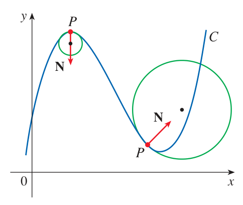
The curvature of a space curve is defined as the rate of change of the unit tangent vector with respect to distance traveled.

For curves in the plane, a single quantity, the angle of inclination $\theta (t)$, is sufficient to characterize the heading direction, and the curvature is given by $\frac{d\theta }{ds}$. For curves in space, the unit vector $\mathbf{T}(t)$ plays the role of $\theta (t)$, giving the heading direction. (In spherical coordinates, a point on the unit sphere is determined by two angle quantities $\theta$, $\phi$.) The rate of change of heading is best described as a vector quantity whose norm gives the curvature:

$$\kappa (t)=\left|\frac{d\mathbf{T}}{ds}(t)\right|=\left|\frac{d\mathbf{T}}{dt}\cdot \frac{1}{s^{\prime }(t)}\right|=\frac{1}{v(t)}|{\mathbf{T}}^{\prime }(t)|.$$

The curvature quantifies a geometrical property of the curve image, and it does not depend on the parametrization. This follows because $\mathbf{T}$ and $s$ are both functions of the curve image. (Plus a chosen direction of travel along the curve that determines signs, but the sign of $\mathbf{T}$ cancels the sign of $s$). A point on the curve may be specified by the parameter $t$ or by the arc length $s$, so $\kappa$ may be considered a function of $t$ or of $s$.

Using the fact that $\mathbf{N}(t)=\frac{1}{|{\mathbf{T}}^{\prime }(t)|}{\mathbf{T}}^{\prime }(t)$, we find that the rate of change of the unit tangent with respect to the parameter can be expressed in terms of speed, curvature, and the unit normal:

$${\mathbf{T}}^{\prime }(t)=v(t)\kappa (t)\mathbf{N}(t).$$ Link to original

Exercise

04

Curvature of a line

Use $\mathbf{r}(t)=(x_0,y_0,z_0)+t\mathbf{v}$ for a vector-valued parametric line. Compute the curvature of this line using the definition of curvature.

Link to original

Exercise

05

Curvature of a circle

Write component formulas for a vector-valued parametric circle of radius $R$ in ${\mathbb{R}}^3$. Compute the curvature of this circle using the definition of curvature.

Link to original

Acceleration decomposition

Acceleration decomposition

The acceleration vector of $\mathbf{r}(t)$ is defined as its second derivative with respect to time: $\mathbf{a}(t):={\mathbf{r}}^{\prime \prime }(t)$.

Since $\mathbf{N}(t)$ is defined using ${\mathbf{T}}^{\prime }(t)$, and $\mathbf{T}(t)$ is defined using ${\mathbf{r}}^{\prime }(t)$, we expect a relation between $\mathbf{N}(t)$ and ${\mathbf{r}}^{\prime \prime }(t)$. Indeed we have:

$${\mathbf{r}}^{\prime \prime }(t)=v^{\prime }(t)\mathbf{T}(t)+(\kappa (t)v(t{)}^2)\mathbf{N}(t).$$

This follows because ${\mathbf{r}}^{\prime }(t)=|{\mathbf{r}}^{\prime }(t)|\mathbf{T}(t)=v(t)\mathbf{T}(t)$, so the product rule gives:

$$\begin{array}{rl}{\mathbf{r}}^{\prime \prime }(t)& =v^{\prime }(t)\mathbf{T}(t)+v(t){\mathbf{T}}^{\prime }(t)\\ & =v^{\prime }(t)\mathbf{T}(t)+(v(t{)}^2\kappa (t))\mathbf{N}(t).\end{array}$$

Efficient curvature formula
The quantity $|{\mathbf{r}}^{\prime }(t)|$ in the denominator of $\mathbf{T}(t)$ often makes the derivative ${\mathbf{T}}^{\prime }(t)$ annoying to compute. It is possible to avoid this derivative by using further reasoning to develop an alternate formula for $\kappa (t)$. First, observe that:

$${\mathbf{r}}^{\prime }(t)\times {\mathbf{r}}^{\prime \prime }(t)=0+v(t)\mathbf{T}(t)\times (\kappa (t)v(t{)}^2)\mathbf{N}(t)=v(t{)}^3\kappa (t)\mathbf{B}(t).$$

Since $\mathbf{B}$ is a unit vector, it follows by taking norms that:

$$\kappa (t)=\frac{|{\mathbf{r}}^{\prime }(t)\times {\mathbf{r}}^{\prime \prime }(t)|}{|{\mathbf{r}}^{\prime }(t){|}^3}.$$

Efficient formula for $\mathbf{N}$
The decomposition of ${\mathbf{r}}^{\prime \prime }(t)$ can also be used to give an efficient formula for $\mathbf{N}$:

$$\mathbf{N}(t)=\frac{v(t){\mathbf{r}}^{\prime \prime }(t)-v^{\prime }(t){\mathbf{r}}^{\prime }(t)}{|v(t){\mathbf{r}}^{\prime \prime }(t)-v^{\prime }(t){\mathbf{r}}^{\prime }(t)|}.$$

We can see this by multiplying the decomposition by $v(t)$:

$$\begin{array}{rl}v(t){\mathbf{r}}^{\prime \prime }(t)& =v^{\prime }(t)v(t)\mathbf{T}(t)+v^{\prime }(t)v(t{)}^2\kappa (t)\mathbf{N}(t)\\ v^{\prime }(t)v(t{)}^2\kappa (t)\mathbf{N}(t)& =v(t){\mathbf{r}}^{\prime \prime }(t)-v^{\prime }(t){\mathbf{r}}^{\prime }(t).\end{array}$$

Dividing both sides by the norm gives the desired formula.

Link to original

Exercise

06

Curvature of a helix

Compute the curvature of the helix given parametrically by $(r\cos (t),r\sin (t),at)$ using the efficient formula. Also compute the unit tangent and principal normal vectors, $\mathbf{T}(t)$ and $\mathbf{N}(t)$. Compute $\mathbf{N}$ once using the definition, and again using the efficient formula.

Link to original

Exercise

07

Curvature of a graph

Use the efficient formula for curvature to derive a formula for the curvature of the graph of a function $f:\mathbb{R}\to \mathbb{R}$, namely the points $(x,y)$ satisfying $y=f(x)$. Start by finding a parametric curve whose image is this graph.

Link to original

Exercise

08

Normal vector to $(t,e^t,t)$ at $t=1$

Compute the principal normal $\mathbf{N}(t)$ using the efficient formula for the parametric curve given by $(t,e^t,t)$ at the point $t=1$.

Link to original

Acceleration decomposition (part 2)

Acceleration decomposition
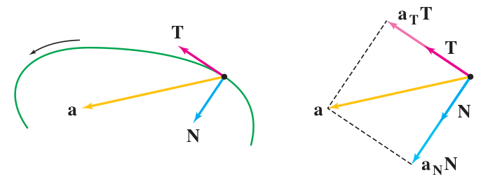
Given that $\mathbf{T}$ and $\mathbf{N}$ are orthogonal unit vectors and ${\mathbf{r}}^{\prime \prime }(t)$ is a linear combination of them, it is appropriate to name the components of ${\mathbf{r}}^{\prime \prime }(t)$ according to the decomposition:

$${\mathbf{r}}^{\prime \prime }(t)=\mathbf{a}(t)=a_{\mathbf{T}}\mathbf{T}+a_{\mathbf{N}}\mathbf{N}.$$

with $a_{\mathbf{T}}:=v^{\prime }(t)$ and $a_{\mathbf{N}}:=\kappa (t)v(t{)}^2$. So $a_{\mathbf{T}}$ is the component of acceleration in the direction of travel, which by the definition is also just the rate of change $v^{\prime }(t)$ of the scalar speed $v(t)$ with respect to time; and $a_{\mathbf{N}}$ is the component of acceleration in the normal direction, perpendicular to the direction of travel.

Acceleration lies in span of $\mathbf{T}$ and $\mathbf{N}$

The fact that $\mathbf{a}$ can be written as a linear combination of $\mathbf{T}$ and $\mathbf{N}$ says something about $\mathbf{N}$. In fact it gives a way to characterize $\mathbf{N}$: it is the unique direction perpendicular to $\mathbf{T}$ that is determined by the part of $\mathbf{a}$ perpendicular to $\mathbf{T}$.

Link to original

Exercise

09

Acceleration on a circle

Write a parametric curve traversing a circle of radius $R$ in ${\mathbb{R}}^3$ at constant speed. Compute the decomposition of acceleration into components: $\mathbf{a}=a_{\mathbf{T}}\mathbf{T}+a_{\mathbf{N}}\mathbf{N}$.

Link to original

Acceleration decomposition (part 3)

Going deeper

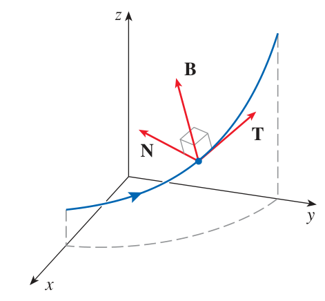
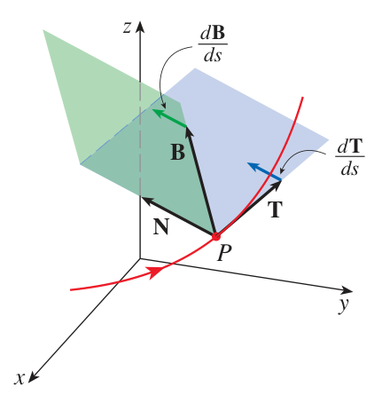
The space of vectors perpendicular to $\mathbf{T}$ is a plane, so $\mathbf{N}$ is not unique with the property that $\mathbf{N}\perp \mathbf{T}$. It is unique in containing the new direction of $\mathbf{a}$. The plane given by all linear combinations of $\mathbf{T}$ and $\mathbf{N}$ is called the osculating plane.

Another unit vector $\mathbf{B}(t)$ may be defined by $\mathbf{B}=\mathbf{T}\times \mathbf{N}$, and we also have $\mathbf{B}\perp \mathbf{T}$. It is called the ‘binormal’ vector. The collection of pairwise orthogonal unit vectors $\mathbf{T},\mathbf{N},\mathbf{B}$ forms a special basis naturally arising from the parametric curve $\mathbf{r}(t)$ which is called the ‘Frenet-Serret frame’, or sometimes the ‘$\mathbf{T},\mathbf{N},\mathbf{B}$ frame’.

Frenet-Serret graphics on Wikipedia

Link to original

Parametric space curves: integration

Arc length parametrization

Arc length parametrization

A parametric curve $\mathbf{r}(t)$ is said to have unit speed when $|{\mathbf{r}}^{\prime }(t)|=1$.

Another description with the same meaning is to say that $\mathbf{r}(t)$ has an arc length parametrization. This terminology is used because the distance-traveled function is $s(t)=t$ when $|{\mathbf{r}}^{\prime }(t)|=1$.

Typically a parametric curve with arc length parametrization is written using the letter ‘$s$’ for the parameter, as in $\mathbf{r}(s)$, to emphasize the fact that the parameter also measures the distance traveled along the curve.

The distance traveled $s$ is also the only natural parameter, in that it is determined by the image curve in ${\mathbb{R}}^3$, whereas any other parameter $t$, for $t\ne s$, suffers from an undesirable arbitrariness. (For example, what geometric reason could be given to choose $t$ instead of $2t+1$?)

A consequence of the fact that $s$ is geometrically natural is that arc length parametrizations are very useful in abstract mathematics, where arguments about geometrical structure are sought. Unfortunately it is often impracticable to create arc length parametrizations with explicit formulas, so they are less useful in practical applications. There are some exceptions.

$$\left|\frac{d}{ds}\mathbf{r}(g(s))\right|=1.$$Link to original

Example

Arc length parametrization of a line

Arc length parametrization of a line.

Calculate an arc length parametrization of the line in the plane given by $y=mx$.

Solution: We create a natural parametrization of the line using $\mathbf{r}(t)=(t,mt)$. Observe that ${\mathbf{r}}^{\prime }(t)=(1,m)$ and $|{\mathbf{r}}^{\prime }(t)|=\sqrt{1+m^2}$. Using the definition of $s(t)$, we then find:

$$s(t)={\int }_0^t\sqrt{1+m^2}du=t\sqrt{1+m^2}.$$

Solving for $t$, we find $t=s\frac{1}{\sqrt{1+m^2}}$. Plugging this into the original parametrization, obtain: $\mathbf{r}(s)=\left(s\frac{1}{\sqrt{1+m^2}},s\frac{m}{\sqrt{1+m^2}}\right).$

Link to original

Exercise

01

Compute arc length parametrization of a helix

Calculate an arc length parametrization of the helix given parametrically by $(\cos (4t),\sin (4t),3t)$. Start by computing the distance-traveled function $s=s(t)$, and then find its inverse function $t=t(s)$, and plug this into the original parametrization.

Link to original

Parametric space curves: vector integration

Vector integrals

Vector integrals

A parametric space curve $\mathbf{r}(t)=(x(t),y(t),z(t))$ has a definite vector integral that is defined componentwise:

$${\int }_a^b\mathbf{r}(t)dt=\left({\int }_a^{b}x(t)dt,{\int }_a^{b}y(t)dt,{\int }_a^{b}z(t)dt\right).$$

The vector integral relates directly to the componentwise derivative ${\mathbf{r}}^{\prime }(t)$ by a vector form of the Fundamental Theorem of Calculus:

$${\int }_a^b\mathbf{r}(t)dt=\mathbf{R}(b)-\mathbf{R}(a)$$

where $\mathbf{R}(t)$ is a vector antiderivative of $\mathbf{r}(t)$, meaning that ${\mathbf{R}}^{\prime }(t)=\mathbf{r}(t)$.

Using the standard calculus argument applied to each component separately, one has the fact that:

$${\mathbf{R}}_1^{\prime }(t)={\mathbf{R}}_1^{\prime }(t)⟹{\mathbf{R}}_1(t)={\mathbf{R}}_1(t)+\mathbf{c},$$

where $\mathbf{c}=(c_1,c_2,c_3)$ is some constant vector. This means that if ${\mathbf{R}}^{\prime }(t)=\mathbf{r}(t)$, so $\mathbf{R}(t)$ is a particular antiderivative of $\mathbf{r}(t)$, then the general antiderivative is given by $\mathbf{R}(t)+\mathbf{c}$ for a constant vector $\mathbf{c}$. So we can write the indefinite vector integral:

$$\int \mathbf{r}(t)dt=\mathbf{R}(t)+\mathbf{c}.$$

The vector integral ${\int }_a^{b}v(t)dt$ may be interpreted as the total motion of a particle whose velocity is given by $v(t)$.

Integration for components, not coordinates

If a parametric curve is given using spherical coordinate functions, for example $(r(t),\theta (t),\phi (t))$, then the componentwise derivatives and integrals do not have vector interpretations as tangent vector and total motion vector. The meaning of vector derivative and integral depends on the componentwise addition and scaling operations applicable to vectors.

Link to original

Example

Indefinite vector integral calculation

Indefinite vector integral calculation

Problem: Compute the indefinite vector integral: $\int (e^t,t^{\frac{1}{2}},\cos (t))dt$.

Solution: The vector integral is given by computing ordinary integrals in each component. We have:

$$\begin{array}{rl}\int (e^t,t^{\frac{1}{2}},\cos (t))dt& =\left(\int e^{t}dt,\int t^{\frac{1}{2}}dt,\int \cos (t)dt\right)\\ & =\left(e^t+c_1,\frac{2}{3}{t}^{\frac{3}{2}}+c_2,\sin (t)+c_3\right)\\ & =\left(e^t,\frac{2}{3}{t}^{\frac{3}{2}},\sin (t)\right)+\mathbf{c}.\end{array}$$

Link to original

Exercise

01

Indefinite vector integrals

Compute the indefinite vector integrals:

• (a) $\int \frac{1}{1+t^2}{\mathbf{e}}_{\mathbf{i}}+t{e}^{t^2}{\mathbf{e}}_{\mathbf{j}}+\sqrt{t}{\mathbf{e}}_{\mathbf{k}}dt$
• (b) $\int (t\cos (t^2),t^{-1},{\sec }^2(t))dt$

Link to original

Exercise

02

Definite vector integrals

Compute the definite vector integrals:

• (a) ${\int }_a^b(1,t^2,\sin (t))dt$
• (b) ${\int }_0^1\left(\frac{1}{1+s^2},\frac{s}{1+s^2}\right)ds$
• (c) ${\int }_0^{1}t{e}^{-t^2}{\mathbf{e}}_{\mathbf{i}}+t\ln (t^2+1){\mathbf{e}}_{\mathbf{j}}dt$
• (d) ${\int }_0^t(3s,6s^2,9)ds$

Link to original

Position, velocity, acceleration

Position, velocity, acceleration

If the position of a moving particle is identified using the vector-valued parametric function $\mathbf{r}(t)$, then its velocity is given by ${\mathbf{r}}^{\prime }(t)$ and its vector acceleration is ${\mathbf{r}}^{\prime \prime }(t)$.

The definite vector integral reverses this progression. We have ${\int }_a^b{\mathbf{r}}^{\prime \prime }(t)dt={\mathbf{r}}^{\prime }(b)-{\mathbf{r}}^{\prime }(a)$, the total change in velocity over the time interval $a\le t\le b$. Similarly ${\int }_a^b{\mathbf{r}}^{\prime }(t)dt=\mathbf{r}(b)-\mathbf{r}(a)$, the total change in position over the same interval.

Link to original

Particle position from velocity - differential equation

Particle position from velocity: differential equation

Problem: Suppose that the path of a particle is given by $\mathbf{r}(t)$ and that its velocity satisfies ${\mathbf{r}}^{\prime }(t)=(1-6\sin (3t),4t,e^t)$, and suppose the particle passes through the point $(4,1,2)$ at $t=0$. Find $\mathbf{r}(t)$ and use your formula to find the position of the particle at $t=2$.

Solution: By taking the indefinite vector integral of both sides of ${\mathbf{r}}^{\prime }(t)=(1-6\sin (3t),4t,e^t)$, we obtain the general solution:

$$\mathbf{r}(t)=\left(t+2\cos (3t),2t^2,e^t\right)+\mathbf{c}.$$

We can solve for $\mathbf{c}$ by setting $\mathbf{r}(0)=(4,1,2)$:

$$(4,1,2)=(2,0,1)+\mathbf{c}$$

so $\mathbf{c}=(2,1,1)$ gives the particular solution satisfying the initial condition $\mathbf{r}(0)=(4,1,2)$.

Link to original

Exercise

03

Differential equations

For the differential equations below, find the general solution, and find the particular solution that satisfies the given initial condition:

• (a) $\frac{d\mathbf{r}}{dt}=(1-3t,4t),\mathbf{r}(0)=(3,1)$
• (b) ${\mathbf{r}}^{\prime }=t^2{\mathbf{e}}_{\mathbf{i}}+5t{\mathbf{e}}_{\mathbf{j}}+{\mathbf{e}}_{\mathbf{k}},\mathbf{r}(1)={\mathbf{e}}_{\mathbf{j}}+2{\mathbf{e}}_{\mathbf{k}}$
• (c) ${\mathbf{r}}^{\prime \prime }(t)=(e^{2t-2},t^2-1,2),\mathbf{r}(0)=(1,0,0),{\mathbf{r}}^{\prime }(0)=(0,1,0)$

Link to original

Kepler’s Law of Ellipses

Kepler’s Law of Ellipses

Isaac Newton’s laws of motion were used to derive and explain Johannes Kepler’s observed law that planets orbit the sun with elliptical orbits. We can use vector integration to solve a differential equation coming from Newton’s laws to give a modern derivation of this law of elliptical orbits.

Set the sun at the origin $(0,0,0)$, and let $\mathbf{r}(t)$ describe the orbit of some planet. Let $G$ be the gravitational constant, $M$ the mass of the sun, and $m$ the mass of the planet. Let $\mathbf{F}(t)$ be the total force vector on the planet. By Newton’s law of gravitation:

$$\mathbf{F}=-\frac{GMm}{|\mathbf{r}{|}^2}{\mathbf{e}}_{\mathbf{r}}.$$

By Newton’s law of motion, $\mathbf{F}=m\mathbf{a}$ where the acceleration is $\mathbf{a}(t)={\mathbf{r}}^{\prime \prime }(t)$. By identifying the force in each equation, we obtain the vector differential equation:

$${\mathbf{r}}^{\prime \prime }(t)=-\frac{GM}{|\mathbf{r}(t){|}^2}{\mathbf{e}}_{\mathbf{r}}(t)=-\frac{GM}{|\mathbf{r}(t){|}^3}\mathbf{r}(t).$$ Link to original

Exercise

04

Prepare to explain the following reasoning in class:

Planet motion stays in some plane: $\mathbf{r}\times {\mathbf{r}}^{\prime }=\mathbf{n}$

Consider the following calculation:

$$\begin{array}{rl}\frac{d}{dt}(\mathbf{r}\times {\mathbf{r}}^{\prime })& ={\mathbf{r}}^{\prime }\times {\mathbf{r}}^{\prime }+\mathbf{r}\times {\mathbf{r}}^{\prime \prime }\\ & =0+\mathbf{r}\times \left(-\frac{GM}{|\mathbf{r}{|}^3}\mathbf{r}\right)=0.\end{array}$$

By integrating both sides of this vector equation, we find $\mathbf{r}\times {\mathbf{r}}^{\prime }=\mathbf{n}$ for some constant vector $\mathbf{n}$. So $\mathbf{n}$ is perpendicular to $\mathbf{r}(t)$ for all $t$, which means $\mathbf{r}(t)$ lies in the plane through the origin with normal vector $\mathbf{n}$.

Link to original

Exercise

05

Prepare to explain the following reasoning in class:

Equation to integrate: $({\mathbf{r}}^{\prime }\times \mathbf{n}{)}^{\prime }=GM{\mathbf{e}}_{\mathbf{r}}^{\prime }$

Next we verify this equation. The product rule gives $({\mathbf{r}}^{\prime }\times \mathbf{n}{)}^{\prime }={\mathbf{r}}^{\prime \prime }\times \mathbf{n}$. Now compute this using the vector differential equation and the definition of $\mathbf{n}$:

$${\mathbf{r}}^{\prime \prime }\times \mathbf{n}=-\frac{GM}{|\mathbf{r}{|}^3}\mathbf{r}\times (\mathbf{r}\times {\mathbf{r}}^{\prime }).$$

Expand the triple product with the Lagrange triple product identity $\mathbf{a}\times (\mathbf{b}\times \mathbf{c})=\mathbf{b}(\mathbf{a}\cdot \mathbf{c})-\mathbf{c}(\mathbf{a}\cdot \mathbf{b})$, and let $r=|\mathbf{r}|$, so $\mathbf{r}=r{\mathbf{e}}_{\mathbf{r}}$, and calculate:

$$\begin{array}{rl}-\frac{GM}{|\mathbf{r}{|}^3}\mathbf{r}\times (\mathbf{r}\times {\mathbf{r}}^{\prime })& =-\frac{GM}{r^3}\left(\mathbf{r}(\mathbf{r}\cdot {\mathbf{r}}^{\prime })-{\mathbf{r}}^{\prime }(\mathbf{r}\cdot \mathbf{r})\right)\\ & =-\frac{GM}{r^3}\left(r{\mathbf{e}}_{\mathbf{r}}(r{\mathbf{e}}_{\mathbf{r}}\cdot (r^{\prime }(t){\mathbf{e}}_{\mathbf{r}}+r{\mathbf{e}}_{\mathbf{r}}^{\prime }))-(r^{\prime }(t){\mathbf{e}}_{\mathbf{r}}+r{\mathbf{e}}_{\mathbf{r}}^{\prime })r^2\right)\\ & =-\frac{GM}{r}\left({\mathbf{e}}_{\mathbf{r}}(r^{\prime }(t)+0)-r^{\prime }(t){\mathbf{e}}_{\mathbf{r}}-r{\mathbf{e}}_{\mathbf{r}}^{\prime }\right)\\ & =GM{\mathbf{e}}_{\mathbf{r}}^{\prime }.\end{array}$$

Link to original

Exercise

06

Prepare to explain the following reasoning in class:

Result of integration: ${\mathbf{r}}^{\prime }\times \mathbf{n}=GM{\mathbf{e}}_{\mathbf{r}}+\mathbf{c}$

Take the indefinite vector integral on both sides of $({\mathbf{r}}^{\prime }\times \mathbf{n}{)}^{\prime }=GM{\mathbf{e}}_{\mathbf{r}}^{\prime }$ and obtain ${\mathbf{r}}^{\prime }\times \mathbf{n}=GM{\mathbf{e}}_{\mathbf{r}}+\mathbf{c}$ where $\mathbf{c}$ is some constant vector.

Notice that $\mathbf{c}\perp \mathbf{n}$ by taking $-\cdot \mathbf{n}$ on both sides of the stated equation, using that ${\mathbf{e}}_{\mathbf{r}}\perp \mathbf{n}$. This means $\mathbf{c}$ lies in the same plane of the orbit that $\mathbf{r}(t)$ lies in.

Let $c:=|\mathbf{c}|$ and let $\theta (t)$ be the angle between $\mathbf{r}(t)$ and $\mathbf{c}$ in the plane perpendicular to $\mathbf{n}$. Also let $n:=|\mathbf{n}|$.

Link to original

Exercise

07

Prepare to explain the following reasoning in class:

Triple product for scalar equation

We take the dot product $\mathbf{r}\cdot -$ on both sides of the previous stated equation, and rearrange the triple product, in order to find a scalar equation:

$$\begin{array}{rl}\mathbf{r}\cdot ({\mathbf{r}}^{\prime }\times \mathbf{n})& =GM\mathbf{r}\cdot {\mathbf{e}}_{\mathbf{r}}+\mathbf{r}\cdot \mathbf{c}\\ \mathbf{n}\cdot (\mathbf{r}\times {\mathbf{r}}^{\prime })& =GMr+rc\cos (\theta ).\end{array}$$

Since $\mathbf{r}\times {\mathbf{r}}^{\prime }=\mathbf{n}$ and $\mathbf{n}\cdot \mathbf{n}=n^2$, we have:

$$n^2=r(GM+c\cos (\theta )),$$

so:

$$r=\frac{n^2}{GM}\left(\frac{1}{1+e\cos (\theta )}\right),$$

where $e:=\frac{c}{GM}$ is defined to simplify the expression. This, now, is the polar equation of an ellipse with eccentricity $e$.

Link to original

Line integrals I: scalar fields

Introduction

A scalar line integral is the integral of a function over the length of a curve.

A line integral sums the values of a scalar function on space multiplied over the length of some curve in space. This would be an ordinary integral if the curve were stretched out onto an $x$-axis and the function values plotted on the $y$-axis.

Line integral with parametrization $\mathbf{r}(t)$
Suppose $f:{\mathbb{R}}^3\to \mathbb{R}$ is a function on space with values given by $f(x,y,z)$, where $(x,y,z)$ are the coordinates of the input point in space. Suppose a curve $C$ is the image of a parametric curve given with component functions by $\mathbf{r}(t)=(x(t),y(t),z(t))$, and assume $C$ is traversed exactly once by $\mathbf{r}(t)$. Then we compute the line integral of $f$ over $C$ using the formula:

$${\int }_{C}f(x,y,z)ds={\int }_a^{b}f(\mathbf{r}(t))\cdot |{\mathbf{r}}^{\prime }(t)|dt.$$

This formula uses our expression for infinitesimal distance traveled:

$$ds=|{\mathbf{r}}^{\prime }(t)|dt=\sqrt{x^{\prime }(t{)}^2+y^{\prime }(t{)}^2+z^{\prime }(t{)}^2}dt.$$

Rigorous definition idea
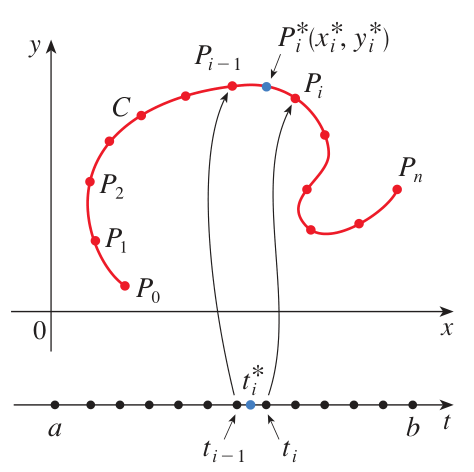
A rigorous definition of the line integral ${\int }_{C}fds$ would divide the curve $C$ into $n$ segments joined at the points $(x_i,y_i,z_i)$, with segment length $\Delta s_i$, then take the Riemann sum:

$$\sum _{i=1}^{n}f(x_i,y_i,z_i)\Delta s_i,$$

and finally take the limit as the number of segments goes to infinity.

Line integral with arc length parametrization
If we start with a curve $\mathbf{r}(s)$ parametrized by arc length, the line integral is very simply given by:

$${\int }_{C}fds={\int }_a^{b}f(\mathbf{r}(s))ds,$$

where $f$ is a scalar function of points in ${\mathbb{R}}^3$.

In fact, the line integral ${\int }_{C}fds$ is sometimes called the line integral with respect to arc length.

Line integral with respect to $x$, $y$, or $z$
A related construction is the line integral with respect to some coordinate. For example, the line integral of $f$ over a curve $C$ with respect to $x$ is given by the formula:

$${\int }_{C}fdx={\int }_a^{b}f(\mathbf{r}(t))\cdot x^{\prime }(t)dt.$$

Sometimes a sum of such integrals is written with shorthand notation as a single integral:

$${\int }_{C}fdx+gdy={\int }_a^{b}f(\mathbf{r}(t))\cdot x^{\prime }(t)+g(\mathbf{r}(t))\cdot y^{\prime }(t)dt.$$

When $C$ is traversed by $\mathbf{r}(t)$, this shorthand can be remembered with formulas using Leibniz notation:

$$dx=x^{\prime }(t)dt,dy=y^{\prime }(t)dt,dz=z^{\prime }(t)dt.$$Link to original

Example

Line integral in the plane

Line integral in the plane

Problem: Compute the line integral:

$${\int }_{C}ydx+zdy+xdz$$

where $C$ is the line segment with endpoints $(2,0,0)$ and $(3,4,5)$.
Solution: We use the formula $\mathbf{r}(t)=(1-t){\mathbf{r}}_0+t{\mathbf{r}}_1$ for a line passing through ${\mathbf{r}}_0$ and ${\mathbf{r}}_1$. This gives $\mathbf{r}(t)=(2+t,4t,5t)$. We also have $dx=dt$, $dy=4dt$, $dz=5dt$. Plugging everything in:

$${\int }_{C}ydx+zdy+xdz={\int }_0^{1}4t+5t\cdot 4+(2+t)\cdot 5dt={\int }_0^{1}10+29tdt=\mathrm{24.5.}$$

Link to original

Example

Total mass of parabolic cable

Total mass of parabolic cable

Problem: A cable lies in ${\mathbb{R}}^2$ in the shape of a parabola satisfying $y=x^2$. The density of the cable is given by $\rho (x,y)=y/x$. Compute the total mass of the cable between $x=0$ and $x=4$.
Solution: We use the parametrization of the parabola $P$ given by $\mathbf{r}(t)=(t,t^2)$ with $0\le t\le 4$. The total mass $M$ is given by the integral of density over the arc length of the curve:

$$M={\int }_P\rho (x,y)ds={\int }_0^4\rho (t,t^2)\cdot |(1,2t)|dt={\int }_0^{4}t\sqrt{1+4t^2}dt\approx \mathrm{43.6.}$$

Link to original

Exercise

01

Line integrals with respect to arc length

Compute the line integrals of the given function over the specified curve:

• (a) $f(x,y,z)=x^2+y^2+z^2$ over the image of $\mathbf{r}(t)=(\cos (t),\sin (t),t)$ for $0\le t\le \pi$
• (b) $f(x,y)=\sqrt{1+9xy}$ over $y=x^3$ for $0\le x\le 1$
• (c) $f(x,y,z)=2x^2+8z$ over $\mathbf{r}(t)=(e^t,t^2,t)$ for $0\le t\le 1$

Link to original

Exercise

02

Electric potential from charged cable

The electric potential $V_p$ at a point $p=(a,b,c)$ in space is sourced by a charged circular wire with charge density $\rho (x,y,z)=\left(2-\frac{x}{R}\right)$. The wire $C$ is located at $(R\cos (t),R\sin (t),0)$. The potential is given by the line integral:

$$V_p=k{\int }_C\frac{\rho (x,y,z)}{d_p}ds$$

where $k$ is a constant, $d_p$ is the distance from $p$ to $(x,y,z)$, and $C$ is a circle parametrized by $(R\cos (t),R\sin (t),0)$. Find the electric potential at the point $p=(0,0,c)$.

Link to original

Exercise

03

Line integrals compressed notation

Compute the following line integrals in the plane:

• (a) ${\int }_{C}ydx+zdy+xdz$ for $\mathbf{c}(t)=(2+t^{-1},t^3,t^2)$, $0\le t\le 1$
• (b) ${\int }_C\frac{-ydx+xdy}{x^2+y^2}$ for the line segment with endpoints $(1,0)$ and $(0,1)$

Link to original

Exercise

04

Line integrals in the plane

Compute the following line integral in the plane:

$${\int }_C(x+2y)dx+x^{2}dy$$

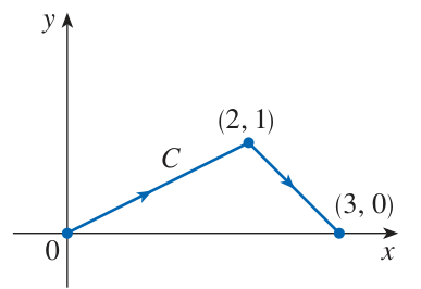
where $C$ is the following curve:

Link to original