Chapter 02 - Qualitative and Numerical Methods

Applications: qualitative behavior

Paths in the plane

Paths in the plane

A classical set of applications of first-order ODEs involves finding paths through space with specific properties.

Link to original

Example

Catenary

Catenary

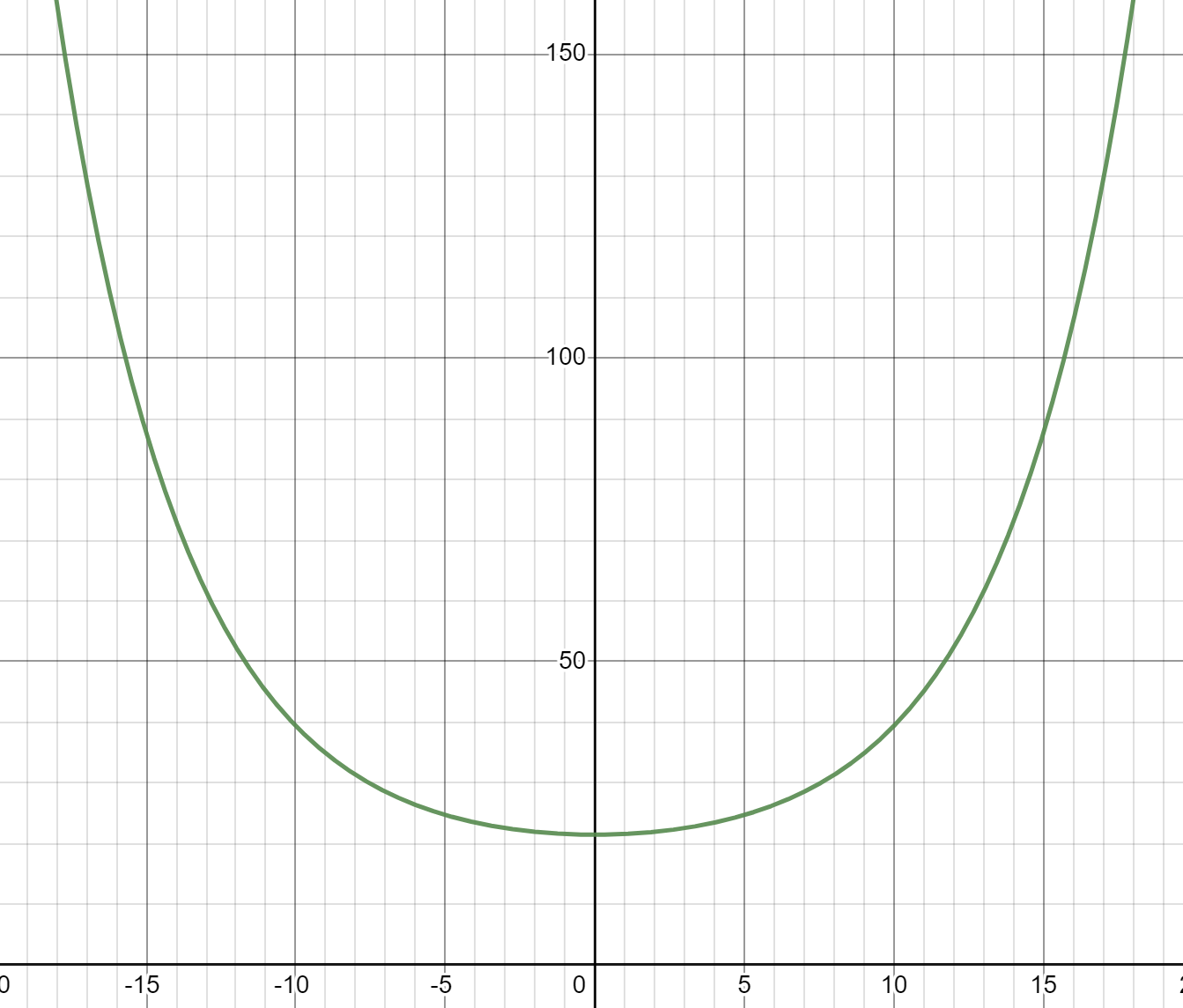
Problem: A catenary is the shape formed by a hanging chain, string, or cable, and also the shape formed by a stable arch. A cable can only resist expansion forces directed along its length, while an arch can only resist compression forces directed along its length. What is the shape of a catenary?

Solution: Consider a hanging chain. Let $F_T$ be the tension force tangent to the chain at a point $p=(x,y)$, and let $F_H$ be the horizontal component of the tension, so $F_H=F_T\cos \theta$, where $\theta$ is the angle formed by the line tangent to the chain at $p$.

The vertical balance of forces is more complicated. Set $x=0$ at the lowest point on the chain, and let $s(x)$ measure the arclength of the chain with $s(0)=0$. At $x=0$, the chain has a horizontal slope, so the vertical component of tension force there is zero. At $p=(x,y)$, the vertical component of tension force is $F_T\sin \theta$. The total vertical force on the portion of chain from the bottom up to $p$ is therefore $F_T\sin \theta$, and this must balance the total weight of the chain from the bottom up to $p$, which is $\rho s(x)$, where $\rho$ is the chain density. So $F_T\sin \theta =\rho s(x)$.

By dividing our two equations, we have $\rho s(x)=F_H\tan \theta$. We may write $\frac{dy}{dx}=\tan \theta$ for the slope of the tangent at $p$. This gives us the differential equation $y^{\prime }=\frac{\rho }{F_H}s(x)$. To solve this, we need to relate the arclength function $s(x)$ to $y(x)$. Recall the arclength formula:

$$s(x)={\int }_{u=0}^x\sqrt{1+(y^{\prime }(u){)}^2}du.$$

Plugging this in gives a differential equation that can be solved algebraically. The solution (family of curves) is:

$$y(x)=\frac{F_H}{\rho }\cosh \left(\frac{\rho }{F_H}x\right)+D.$$

If we set $h_0=y(0)$, i.e. the vertical position of the bottom of the chain, we can solve for $D$ and obtain:

$$y(x)=\frac{F_H}{\rho }\cosh \left(\frac{\rho }{F_H}x\right)+\left(h_0-\frac{F_H}{\rho }\right).$$

https://www.desmos.com/calculator/ngjjfg5yxj

Link to original

Question

01

Solve the ODE

Solve (algebraically) the ODE used to define the catenary curve.
(Hint: differentiate the function $s(x)$, substitute in, then use a reduction of order.)

Link to original

Question

02

Arch vs. chain

Why does the St. Louis arch (or any other self-supporting arch) also have a catenary shape?

Link to original

Example

Tractrix

Tractrix

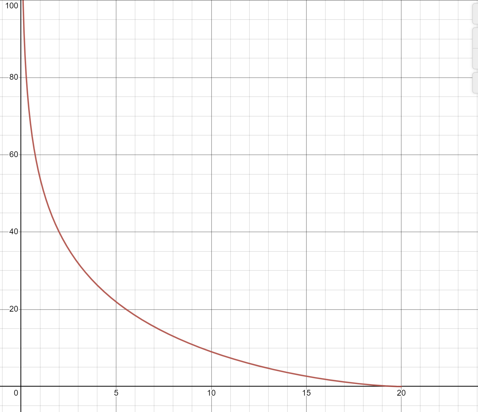
A tractrix is a curve given by dragging a point behind a string of fixed length.

Problem: Suppose we drag the point $p$ behind a string of length $a$. Suppose $p$ starts at $(a,0)$, and we start at $(0,0)$ and walk in the $+y$ direction. What is the shape of the path of $p$?

Solution: Write $p=(x,y)$. The tangent line to the string at $p$ has slope given by

$$\frac{dy}{dx}=-\frac{\sqrt{a^2-x^2}}{x}.$$

To see this, draw the triangle with vertices $(x,y)$ and $(0,y)$ and $(0,y+\sqrt{a^2-x^2})$. The hypotenuse of this triangle is the string itself, and we are pulling from the top vertex.

This equation is separable, and the solution is:

$$y(x)=a\ln \left(\frac{a+\sqrt{a^2-x^2}}{x}\right)-\sqrt{a^2-x^2}.$$

https://www.desmos.com/calculator/9mu1stojhl

Link to original

Question

03

Pushing a pole

Suppose a pole is pushed from one end, with a free pivot on the end from which it is pushed. The shape of the path taken by the opposite end is also a tractrix. Why?

(Describe the concept of tractrix in such a way that it applies equally to dragging strings and pushing poles.)

Link to original

Paths in the plane (part 2)

Catenary vs. tractrix
The catenary curve is the evolute of the tractrix; the tractrix is the involute of the catenary.
https://en.wikipedia.org/wiki/Involute#Involute_and_evolute

Link to original

Example

Pursuit curve

Pursuit curve

Problem: A gazelle runs up the $y$-axis at speed $v_1$ starting at $(0,0)$, and a cheetah runs towards the gazelle at speed $v_2$ starting at $(a,0)$. What is the shape of the path taken by the cheetah?

Solution: The gazelle’s path can be given parametrically by the curve $\mathbf{r}(t)=(0,v_{1}t)$. Suppose the cheetah is at point $p=(x,y(x))$. The vertical distance from cheetah to gazelle is $y-v_{1}t$, and the horizontal distance is $x$.

We assume the cheetah is always running straight toward the gazelle, so the slope of the tangent line to the cheetah’s path is $(y-v_{1}t)/x$, and we obtain the differential equation:

$$\frac{dy}{dx}=\frac{y-v_{1}t}{x}.$$

This equation involves two independent variables, $t$ and $x$, so we cannot immediately solve it. Of course they are related by the fact that $x(t)$ is the $x$-coordinate of the cheetah’s path. We would like to eliminate $t$ from the equation by substituting a formula for $t$ in terms of $x$, $y$, and $y^{\prime }$ quantities. This is the hard part.

We know that the cheetah is running at speed $v_2$, so we also have the equation:

$$v_2=\frac{ds}{dt}=\frac{ds}{dx}\frac{dx}{dt}=-\sqrt{1+(y^{\prime }{)}^2}\frac{dx}{dt}.$$

(Here we use $s(t)$ for the arclength of the cheetah’s path.) This equation relates $t$ to the quantities $x$, $y$, and $y^{\prime }$.

Now we seek to combine the equations. We can flip the second equation to obtain

$$\frac{dt}{dx}=-\frac{1}{v_2}\sqrt{1+(y^{\prime }{)}^2}.$$

If we differentiate the first equation in $x$, we can make the $t$ disappear, with $dt/dx$ appearing instead:

$$\begin{array}{rl}{y}^{\prime \prime }(x)& =\frac{x(y^{\prime }-v_1{t}^{\prime })-(y-v_{1}t)}{x^2}\\ & =\frac{y^{\prime }}{x}-\frac{v_1}{x}\frac{dt}{dx}-\frac{y^{\prime }}{x}\\ & =-\frac{v_1}{x}\frac{dt}{dx}\\ x{y}^{\prime \prime }& =\frac{v_1}{v_2}\sqrt{1+(y^{\prime }{)}^2}.\end{array}$$

Set $k=v_1/v_2$. Reduce the order using $p(x)=y^{\prime }(x)$ and obtain:

$$p(x)=\frac{1}{2}\left({\left(\frac{x}{a}\right)}^k-{\left(\frac{a}{x}\right)}^k\right)$$

Integrate this again to find $y$, solving for the constant using the initial condition $y(a)=0$:

$$y(x)=\frac{1}{2}\left(\left(\frac{a}{k+1}\right){\left(\frac{x}{a}\right)}^{k+1}-\left(\frac{a}{1-k}\right){\left(\frac{x}{a}\right)}^{1-k}\right)+\frac{ak}{(1-k^2)}.$$

https://www.desmos.com/calculator/geosk6qjrb

Link to original

Question

04

Checking algebra

Check the algebra for the solution of $p(x)$ and then the integration for $y(x)$. (Write out all intermediate steps.)

Link to original

Growth and decay

Growth and decay

Another classic application of differential equations produces exponential growth and decay. Variants on this theme can account for recurring additions and subtractions.

Link to original

Example

Growth of retirement fund with compound interest

Growth of retirement fund with compound interest

A quantity of money $A(t)$ in a savings account with compound interest rate $r$ grows according to the differential equation $A^{\prime }(t)=rA$. The solution of this equation is an exponential function $A(t)=A_0{e}^{rt}$, where $A_0=A(0)$ is the initial quantity in the account.

Theory: Compound interest with continuous deposit or withdrawal
Suppose you make continuous deposits or withdrawals at a rate of $d$ (in dollars per year, with $d>0$ for deposits, $d<0$ for withdrawals). Now the equation is:

$$\frac{dA}{dt}=rA+d.$$

This equation is linear and separable. The solution can be found algebraically:

$$A(t)=C{e}^{rt}-\frac{d}{r}.$$

If the account starts with $A(0)=0$, then $C=\frac{d}{r}$ and $A(t)=\frac{d}{r}(e^{rt}-1)$.

Achieving a retirement fund
Suppose this situation describes your Roth IRA. How much should you deposit in the account per year to achieve $800,000 after 40 years, with $r=0.05$? Answer:

$$d=\$800,000\cdot \frac{0.05}{e^{0.05\cdot 40}-1}=\$6261.$$

Constant rate of retirement withdrawal, with inflation
Suppose you have a retirement account with $A_0$ dollars, growing at the interest rate $r$, and you plan to withdraw money at a rate which is increasing with inflation at $k=2\%$ per year, and starting at $80,000 per year. What should $A_0$ be to ensure you will have money for 30 years of retirement?

This problem involves two exponential growths, one stemming from interest and the other from inflation. The rate of withdrawal $W(t)$ satisfies $W^{\prime }(t)=kW$, so $W(t)=W_0{e}^{kt}$ per year. Then the account value satisfies:

$$\frac{dA}{dt}=rA-W_0{e}^{kt}.$$

This equation is linear. The solution is:

$$A(t)=C{e}^{rt}-\frac{W_0}{k-r}{e}^{kt}.$$

Setting $A(0)=A_0$, we can solve for $C$. Then plugging in $A(30)=0$, obtain the equation:

$$\left(A_0+\frac{W_0}{k-r}\right)e^{r\cdot 30}=\frac{W_0}{k-r}{e}^{k\cdot 30}.$$

Setting $W_0=$ $80,000, $r=0.05$, and $k=0.02$, solve for $A_0$ and find $1,580,000.

Link to original

Exercise

01

Design your traditional IRA

You are planning a traditional IRA for retirement: contributions during your working life are pre-tax, and withdrawals during retirement are taxed according to your income bracket when withdrawing. Your plan is to start the fund with $20,000 when you turn 30, and then to contribute a fixed yearly amount $X$ (modeled with a continuous yearly addition rate) each year until you turn 65. You invest the IRA in a broad market index with average yearly returns of 10% (not adjusted for inflation). Starting at age 65 you stop contributing and start withdrawing $70,000 per year after taxes for the next 25 years of retirement, and you would like to have $200,000 remaining in your estate at age 90, both figures measured in today’s dollars. Your tax bracket with this retirement income is 20%. Inflation is assumed to be a steady 2.5% per year. Everything is compounded continuously. What should you choose for the yearly contributions $X$?

Link to original

Example

RC Circuits

RC Circuits

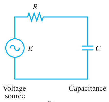
An electrical circuit with a single resistor and a single capacitor is called an RC circuit:

Suppose the voltage source $E$ produces a voltage $V(t)$ between its terminals, and write $V_R$ and $V_C$ for the voltage drops across the resistor and capacitor.

By Ohm’s Law, $V_R=IR$, where $I$ is the current flowing through the resistor, and $R$ is the resistance of the resistor (a constant). The capacitor voltage drop satisfies $V_C=\frac{q}{C}$, where $q$ is the charge stored in the capacitor, and $C$ is the capacitance of the capacitor (a constant). Current is the rate of flow of charge per unit time: $I=\frac{dq}{dt}$.

By Kerchoff’s Voltage Law, we have an equation for the circuit:

$$\begin{array}{rl}V(t)& =V_R+V_C\\ & =IR+\frac{q}{C}.\end{array}$$

So we find that charge satisfies:

$$\begin{array}{rl}\frac{dq}{dt}& =\frac{V(t)-q/C}{R},\\ q^{\prime }(t)+\frac{1}{RC}q(t)& =\frac{1}{R}V(t),\end{array}$$

which is a linear ODE. Solving this ODE and dividing by $C$ gives us a formula for $V_C(t)$:

$$V_C(t)=\frac{1}{C}q(t)=V_0{e}^{-t/RC}+e^{-t/RC}\frac{1}{RC}{\int }_0^t{e}^{s/RC}V(s)ds.$$

Let us study this solution. The first term, $V_0{e}^{-t/RC}$, represents exponential decay from $V_0$ to $0$. The second term depends on the source function $V(t)$. For example, if $V(t)=V$ a constant, then the entire second term reduces to $V$ itself, and the solution $V_C(t)$ will exponentially decay from $V_0+V$ down to $V$.

Here is a Mathlet that shows the response $V_C(t)$ when the source $V(t)$ is a rectangular wave:
https://mathlets.org/mathlets/periodic-box/

Link to original

Exercise

02

Bacteria growth on surface of spherical clump

A spherical clump of bacteria is growing in such a way that only the bacteria on its surface can reproduce, because only these are exposed to new food sources in the environment, while these surface bacteria do reproduce with exponential growth. Recall the formulas for volume and surface area of a sphere:

$$V=\frac{4}{3}\pi r^3,A=4\pi r^2.$$

Find a differential equation satisfied by the number $N(t)$ of bacteria as a function of time.

Link to original

Autonomous equations

Autonomous equations

In a first calculus class, the sign of the derivative $y^{\prime }$ of a function $y(x)$ is written on the number line in order to indicate places where $y$ is increasing or decreasing. This technique is useful for determining whether a critical point is a local min, max, or neither.

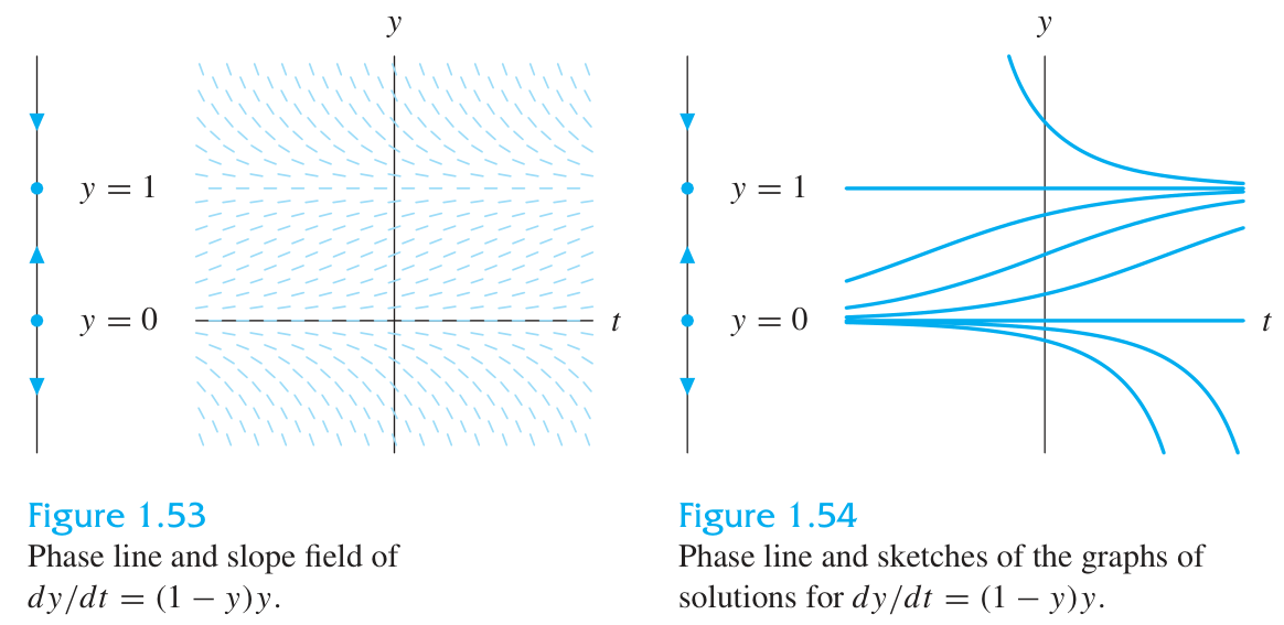
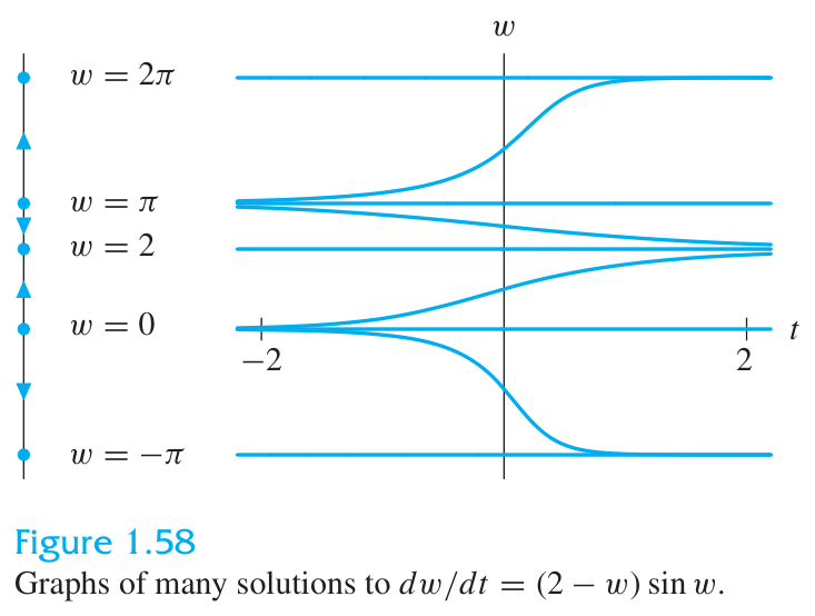
The same technique is used to study first-order autonomous differential equations. Autonomous equations having the form $\frac{dy}{dt}=f(y)$, meaning that the defining function $f$ does not involve the independent variable $t$.

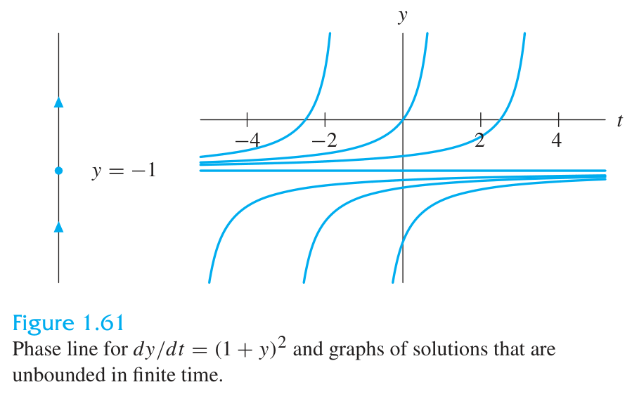
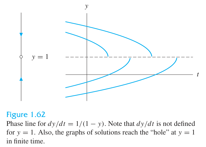
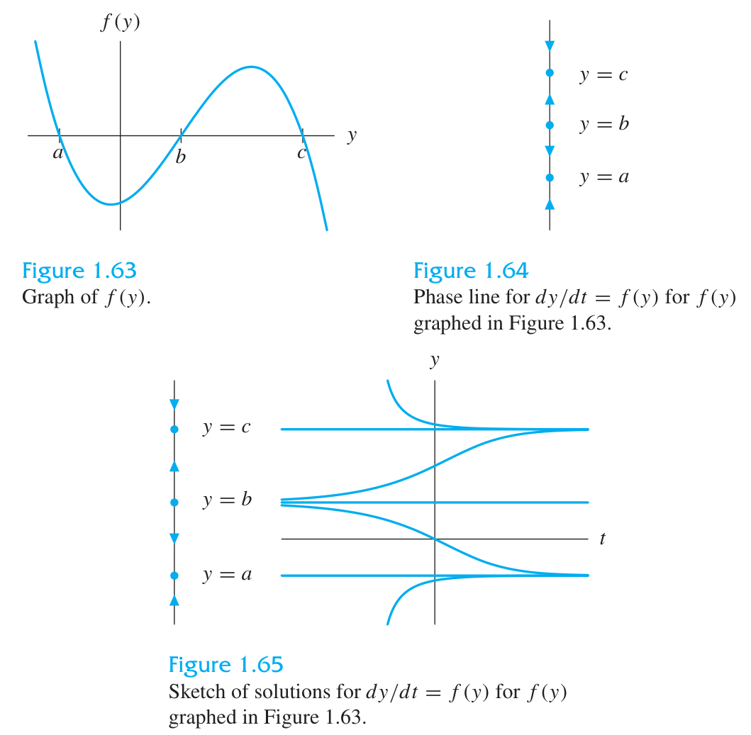
The main differences are: (i) for autonomous ODEs we have the derivative $f(y)$ but we do not already have the function $y(t)$, and (ii) for autonomous ODEs we draw the signs of $f(y)$ as vertical arrows (up or down) on a vertical line, instead of “$+$” and “$-$” on a horizontal line. We can add filled dots where $f(y)=0$, and open dots or dashed lines where $f(y)=\pm \infty$, since these lines have special meaning.

This vertical number line we use to analyze $\frac{dy}{dt}=f(y)$ is called a phase line. Phase lines can be used to make qualitative observations about the behavior of solutions to autonomous ODEs.

Lines $y=y_0$ corresponding to zeros of $f(y)$ yield flat solutions. If the derivative is negative at such a line, i.e. $f^{\prime }(y_0)<0$, so $f(y)$ cross through zero from above to below, then solutions will be attracted to the line $y=y_0$. These lines are called stable equilibria. If $f^{\prime }(y_0)>0$ then solutions will be repelled from the line. These lines are called unstable equilibria. (Sometimes stable equilibria are called sinks and unstable ones which are repulsive on both sides are called sources, while unstable ones that are repulsive on one side and attractive on the other side are called nodes.)

When $f^{\prime }(y_0)=0$, the equilibrium $y=y_0$ could be stable, unstable, or neither, and additional information is needed. The situation is the same as for critical points of a function that fails the second-derivative test.

Phase lines:

Phase lines with $f\to \infty$ at $y=1$:

Phase lines deduced from the graph of $f(y)$ alone:

Logistic growth
Many natural systems experience exponential growth and decay only to first order. Once the exponential behavior has occurred for significant time, environmental effects of the growth or decay begin to modulate the rate of that growth or decay.

Exponential growth satisfies the equation $y^{\prime }(t)=ry$, where $r$ is a constant giving the growth rate. We can modify the equation to account for changes of growth rate that depend on the quantity $y$ by letting $r$ become a function $h(y)$.

Link to original

Example

Logistic curve - population dynamics

Logistic curve: population dynamics

Modified exponential growth with a growth rate given by the linear function $h(y)=r-ay$ gives the logistic equation:

$$\frac{dy}{dt}=(r-ay)y.$$

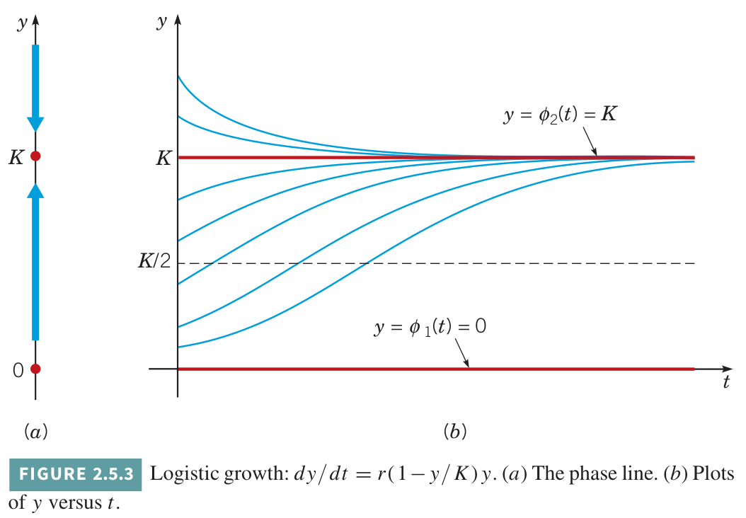
Using the theory of phase lines, we can study solutions to this equation without finding an explicit formula for them. Write $K=r/a$, so $f(y)=r\left(1-\frac{y}{K}\right)y$. This number $K$ is sometimes called the carrying capacity of the population’s environment, because the growth rate $r\left(1-\frac{y}{K}\right)$ will go negative when $y$ exceeds $K$.

Now let us classify equilibrium points. We have $f(0)=f(K)=0$. Compute

$$f^{\prime }(y)=r-2ay=r\left(1-2\frac{y}{K}\right),$$

so $f^{\prime }(0)=r>0$ and $f^{\prime }(K)=-r<0$. Therefore $y=0$ is an unstable equilibrium, while $y=K$ is a stable equilibrium.

The logistic equation is separable, and it can be solved exactly and explicitly. Solutions are called logistic curves. These are given by:

$$y(t)=\frac{y_{0}K}{y_0+(K-y_0)e^{-rt}}.$$

Consider the interpretation of this formula. The initial value is $y(0)=y_0$. As $t\to \infty$, the second term in the denominator goes to zero. So $y(t)\to K$ as $t\to \infty$. This is true whether $y_0>K$ or $y_0<K$.

It is useful to observe that the concavity of the solution trajectories can be ascertained from the formula for $f(y)$ without actually solving the logistic equation. This relies on the chain rule:

$$\frac{d^{2}y}{d{t}^2}=\frac{d}{dt}f(y)=f^{\prime }(y)\frac{dy}{dt}=f^{\prime }(y)f(y).$$

For the logistic equation we are considering, this product is:

$$f^{\prime }(y)f(y)=r^2\left(1-2\frac{y}{K}\right)\left(1-\frac{y}{K}\right)y.$$

The inflection point is where this function changes sign, which is at $y=\frac{1}{2}K$, so the rate of population increase starts slowing down when the population is halfway to the carrying capacity of the environment.

Link to original

Exercise

03

Studying an autonomous equation

Sketch the phase line of the following ODE:

$$\frac{dy}{dt}=(y^2-2)\arctan (y).$$

Classify each equilibrium trajectory as stable or unstable. Draw some representative solution trajectories using the qualitative information of your phase line.

Link to original

Exercise

04

Gompertz equation

Tumor growth is sometimes modeled by the Gompertz equation:

$$\frac{dX}{dt}=aX-bX\ln X.$$

What are the equilibrium lines? Are they stable or unstable? What is the inflection point on a trajectory from the lower to the upper equilibrium?

Now solve the equation explicitly.

Link to original

Numerical techniques

Introduction

This section is about methods that can be used by a computer to produce numerical solutions to first-order IVPs, and more specifically, methods that are usually guaranteed at least some success and rely only on the ability to calculate the derivative $\frac{dy}{dt}$ by evaluating a given function $f(t,y)$. These methods work by starting at the initial value and iteratively building a solution, stepping forward in time to propose candidate $y$ values that depend on evaluations of $f(t,y)$ at various points as well as the $y$ values at previous times.

Extending partial functions in time vs. refining complete functions to higher orders

Later we will consider approximation methods of a different nature, namely power series (for example as produced by Picard iteration), and Fourier series.

Instead of building a solution out across time, producing future solution values during the process, these methods produce coefficients for infinite series that converge to the solution. A systematic approach along these lines was developed by Parker-Sochacki.

The methods of this section produce partial functions defined only up to a given time, and these partial functions are not updated in the past (at least not much), rather they are extended ever further forward. The power series methods produce complete functions, namely as partial sums of the series, but the values at early times are subject to revision as later terms are added, meaning that the complete functions are changed across all time with each further iteration.

Link to original

Euler’s method

Euler’s method

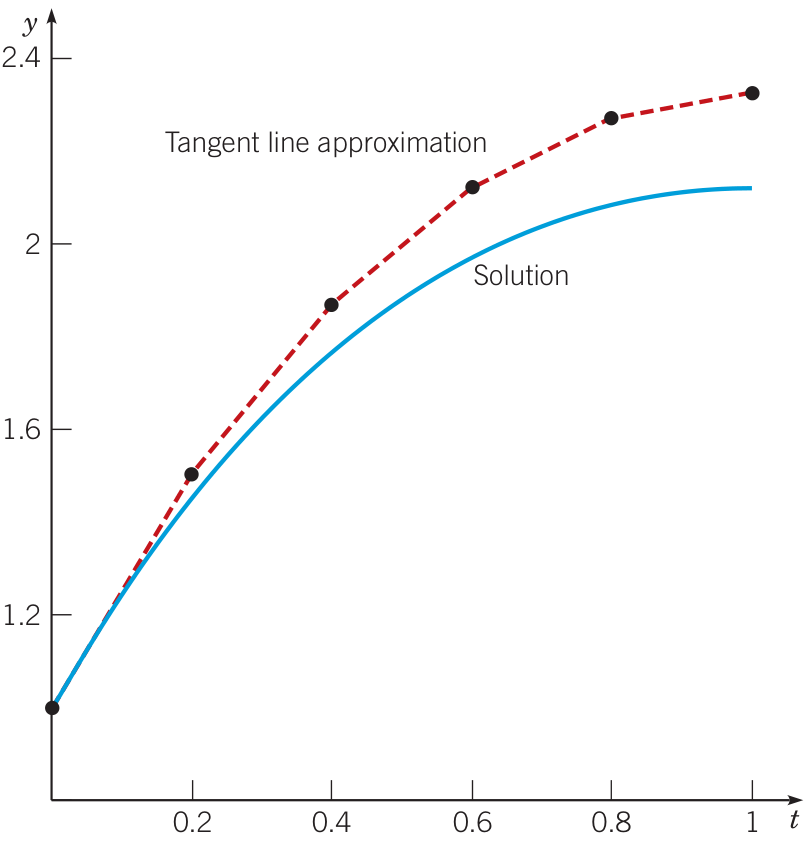
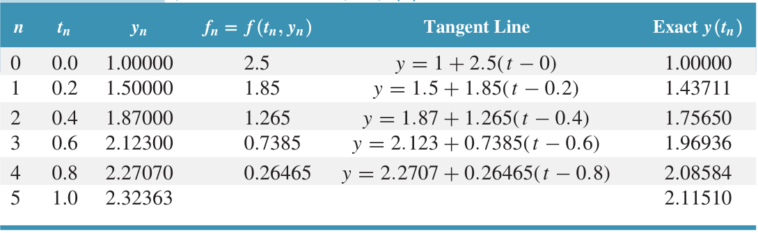
The simplest imaginable algorithm for solving an IVP numerically is attributed to Euler. The method is simply to follow tangent lines.

Suppose the IVP is given by

$$\frac{dy}{dt}=f(t,y),y(t_0)=y_0.$$

We construct an approximate solution iteratively, using a step size of $\Delta t=h$, as follows:

$$\begin{array}{rl}{y}_1& =y_0+hf(t_0,y_0)\\ y_2& =y_1+hf(t_0+h,y_1)\\ y_3& =y_2+hf(t_0+2h,y_2)\\ y_4& =y_3+hf(t_0+3h,y_3)\\ \dots & \dots \\ y_{n+1}& =y_n+hf(t_0+nh,y_n)\end{array}$$

The process is iterated until $t_0+nh$ reaches the desired stopping time $t_N$.

Link to original

Question

01

Euler’s method practice

Consider the IVP:

$$y^{\prime }=2y-3t,y(0)=1.$$

Use Euler’s method to compute an approximate solution up to $t=0.20$ with step size $h=0.05$. Show all four steps of the partial solution.

Link to original

Euler’s method (part 2)

Euler’s method is not always accurate

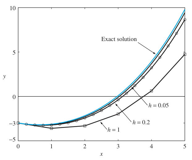
The Euler method is very easy to implement on a computer or even a programmable calculator. It is frequently very inaccurate, however, since the errors can build up rapidly. With exponentially growing solutions, for example, the Euler method will fall far behind in a short time, even with a small step size.

Link to original

Exercise

01

Euler’s method struggles with large slopes

Consider the IVP:

$$y^{\prime }=\frac{3t^2}{3y^2-4},y(1)=0.$$

Desmos: https://www.desmos.com/calculator/gbijdaprd3

• Use Euler’s method to compute an approximate solution at the times $t=1.2,1.4,1.6,1.8$ using $h=0.10$.
• Use Euler’s method to compute an approximate solution at the times $t=1.2,1.4,1.6,1.8$ using $h=0.05$.
• By considering the slope field, possibly in conjunction with an exact solution, can you explain why the approximate solutions differ so much at $t=1.8$?

Link to original

Exercise

02

Euler’s method becomes the left-endpoint rule

Show that if the ODE is amenable to solution by direct integration, meaning $f(t,y)$ actually does not depend on $y$, then Euler’s method amounts to the left-endpoint rule for integration of $f(t)$.

Link to original

Heun’s method

Heun’s method

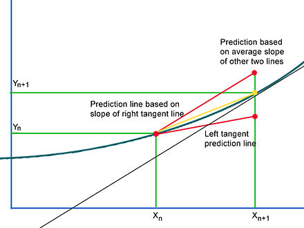
The function $f(t,y)$ allows us to access slope values anywhere, but in Euler’s method we only use the slope value at the starting point of each step.

Instead of taking the slope at $(t_n,y_n)$ to extrapolate from $(t_n,y_n)$, we can take the slope at both $(t_n,y_n)$ and $(t_{n+1},y_{n+1})$. Well, this can’t quite be done because we don’t know $y_{n+1}$ in advance, but we could use the Euler method to forecast $y_{n+1}$ initially and call this $y_{n+1}^{\star }$, then take the slope $f(t_{n+1},y_{n+1}^{\star })$, and finally compute the average slope at the two points. Then we extrapolate our next step from $(t_n,y_n)$ using this average slope instead of the slope $f(t_n,y_n)$. We obtain the formula:

$$y_{n+1}=y_n+h\left(\frac{f(t_n,y_n)+f(t_n+h,y_n+hf(t_n,y_n))}{2}\right).$$

This formula can be iterated from $(t_0,y_0)$ with step size $h$ until reaching the desired stopping time $t_N$.

Link to original

Question

02

Heun’s method practice

Consider the IVP:

$$y^{\prime }=2y-3t,y(0)=1.$$

Use Heun’s method to compute an approximate solution up to $t=0.20$ with step size $h=0.05$. Show all four steps of the partial solution.

Link to original

Question

03

Comparing methods

Solve algebraically the IVP as in the previous Questions: $y^{\prime }=2y-3t,y(0)=1$. Make a table of values to compare the results of Euler’s method, Heun’s method, and the exact solution. Write the percent error next to the values from the approximation methods. Create a final column that includes the percent difference between the approximate solutions. Can this column predict the percent error without knowing the exact solution?

Link to original

Heun’s method (part 2)

Heun’s method becomes the trapezoid rule

If the ODE is amenable to direct integration, so $f(t,y)$ actually does not depend on $y$, then Heun’s method amounts to the trapezoid rule for integration of $f(t)$.

Link to original

Runge-Kutta methods

Runge-Kutta methods

The basic idea of Heun’s method is to capture more information from $f(t,y)$ ahead of the given step $(t_n,y_n)$. We want to use these candidate slope values in the vicinity of the point $(t_n,y_n)$ to better approximate the exact average slope, namely the value that gives the slope of the secant from the current step $(t_n,y_n)$ to the exact solution at the next step.

The idea of Heun’s generalization of Euler’s method can be extended to any number of stages, where a stage refers to the number of ‘forecasting’ evaluations of the function $f(t,y)$ that are required for each step. The Euler method is 1-stage, and the Heun method is 2-stage.

The general name for $n$-stage methods that generalize Heun’s method is Runge-Kutta methods. The most famous and widely used Runge-Kutta method is a choice of 4-stage method that sometimes is simply called the Runge-Kutta method. (So if no stage number is specified, this 4-stage method is implied.)

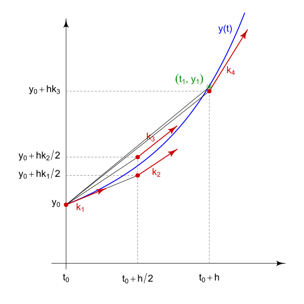
For this method, we sample 4 slope values, called $k_1,\dots ,k_4$:

• $k_1=f(t_n,y_n)$ – slope at current step
• $k_2=f(t_n+\frac{h}{2},y_n+\frac{h}{2}{k}_1)$ – slope at the Euler forecast using $k_1$, half step
• $k_3=f(t_n+\frac{h}{2},y_n+\frac{h}{2}{k}_2)$ – slope at the Euler forecast using $k_2$, half step
• $k_4=f(t_n+h,y_n+h{k}_3)$ – slope at the Euler forecast using $k_3$, full step
  The final value for the next step is then: $$y_{n+1}=y_n+h\left(\frac{k_1+2k_2+2k_3+k_4}{6}\right).$$ In other words, the slope we use to compute the next step $(t_{n+1},y_{n+1})$ is a weighted average of various slopes in the ‘future vicinity’ of $(t_n,y_n)$.

The possibilities are endless

There is no simple explanation for the choice of sampling locations and the choice of weights $(1,2,2,1)$ used for the final slope. Other possibilities are also studied.

Link to original

Exercise

03

The Runge-Kutta method becomes the Simpson rule

Show that if the ODE is amenable to direct integration, so $f(t,y)$ actually does not depend on $y$, then the Runge Kutta method amounts to the Simpson rule for integrating $f(t)$.

Recall that the Simpson rule comes from fitting parabolas. It is given by:

$${\int }_a^{a+h}f(x)dx=\frac{h}{6}(f(a)+4f(a+h/2)+f(a+h)).$$

Link to original

Adams method: multistep: polynomial fitting

Adams method - multistep - polynomial fitting

The methods studied so far, Euler, Heun, and Runge-Kutta more generally, have been single step methods. This terminology means that each step of the iterative process makes use of the data of a single previous step. In the formulas above, $y_{n+1}$ was determined (through some process) by the value of $y_n$ alone.

A multistep method uses the data of multiple previous steps to estimate the next step. For example, a 3-step method would use $y_{n-2}$, $y_{n-1}$, $y_n$ in order to estimate $y_{n+1}$.

Runge-Kutta is not multistep

Do not confuse the use of multiple estimated slopes with the use of multiple previous steps!

To simplify the formulas for multistep methods we define $f_n:=f(t_n,y_n)$, so $f_n$ is a scalar quantity representing the slope given by the ODE at the previous step $y_n$.

The most natural and common multistep method is produced by fitting a polynomial of degree $k$ to the slopes at the $k$ previous steps, namely to

$$f_{n-k+1},f_{n-k+2},\dots ,f_n,$$

and then extrapolating forward on this polynomial. This is called the Adams method.

Link to original

Example

Two-step Adams method

Two-step Adams method

We seek a parabola $g(x)=a{x}^2+bx+c$ with three properties:

$$\begin{array}{rl}g(t_n)& =y_n\\ g^{\prime }(t_n)& =f_n\\ g^{\prime }(t_{n-1})& =f_{n-1}.\end{array}$$

The graph $y=g(x)$ of this parabola will pass through the previous step $(t_n,y_n)$ and match the slope of the ODE at the two previous steps $(t_n,y_n)$ and $(t_{n-1},y_{n-1})$.

To find the coefficients of $g(x)$, first solve the system:

$$\begin{array}{rl}a{t}_n^2+b{t}_n+c& =y_n\\ 2a{t}_n+b& =f_n\\ 2a{t}_{n-1}+b& =f_{n-1}.\end{array}$$

(Observe that the second and third equations are independent of the first, so they should be solved initially and the result used to compute $c$ from the first equation.) Obtain:

$$\begin{array}{rl}a& =\frac{f_n-f_{n-1}}{2h}\\ b& =\frac{f_{n-1}{t}_n-f_n{t}_{n-1}}{h}\\ c& =y_n+\frac{f_n-f_{n-1}}{2h}{t}_n^2-f_n{t}_n.\end{array}$$

Then the next step value $y_{n+1}$ is given by evaluating the polynomial $g(x)$ at $t_{n+1}$:

$$\begin{array}{rl}{y}_{n+1}& =g(t_n+h)\\ & =a(t_n+h{)}^2+b(t_n+h)+c\\ & =(a{t}_n^2+b{t}_n+c)+2a{t}_{n}h+a{h}^2+bh\\ & =y_n+h(f_n-b)+a{h}^2+bh\\ & =y_h+h{f}_n+\frac{1}{2}h(f_n-f_{n-1})\\ & =y_n+\frac{3}{2}h{f}_n-\frac{1}{2}h{f}_{n-1}.\end{array}$$

This is the Adams formula for $y_{n+1}$ in terms of $f_n$ and $f_{n-1}$.

Link to original

Exercise

04

Three-step Adams method

Compute the formula for the three-step Adams method.

Link to original

Errors

Errors

Next we consider the accuracy of the above methods in a quantitative way. It is important to learn some vocabulary to refer to various sources of error, especially as users of numerical ODE solver packages.

• Local truncation error $e_n$ is error arising in the single $n^{\text{th}}$ step of the iterative solution procedure, assuming that the starting values of the previous step are accurate (or taking them for granted as initial conditions).
• Global truncation error $E_n$ is the accumulation of local truncation error as the procedure is iterated over $n$ steps.
• Round-off error $R_n$ is the accumulation of error due to finite-precision arithmetic operations performed along the way, as the procedure is iterated over $n$ steps.
• Total accumulated error $E$ is the difference between the approximate and the exact solutions at the ending time. It is satisfies $|E|\le |E_N|+|R_N|$ where $N$ is the step number of the ending time.

The global truncation error is (in principle) some function of the local truncation error, since it measures the accumulation of that error.

Truncation errors are due to the mathematics of the approximation procedure. For a coherent procedure, the truncation errors should vanish in the limit as $h\to 0$ and the approximation converges to an exact solution. Truncation error is therefore reported in terms of powers of $h$.

The “Big-O” notation $\mathcal{O}(g(h))$ is used to describe how quickly $f(h)\to 0$ as $h\to 0$. The ‘$\mathcal{O}$’ can be read as “order.” We say $f(h)\in \mathcal{O}(g(h))$, read “$f$ has the order of $g$,” when $|f(h)|\le Mg(h)$ for some $M>0$ and $h\to 0$.

With the Euler method, for example, we will see that $e_n\in \mathcal{O}(h^2)$ and $E_n\in \mathcal{O}(h)$, so the Euler method is called a first-order method. It turns out that the Runge-Kutta method has $E_n\in \mathcal{O}(h^4)$, and it is therefore called a fourth-order method. Any method with $E_n\in \mathcal{O}(h^p)$ is at worst a $p^{\text{th}}$-order method. The goal in constructing Runge-Kutta methods is to minimize the number of calls to the function $f(t,y)$ while maximizing the order of the global truncation error.

Local truncation error for the Euler method

Assume that $f,f_t,f_y$ are all continuous in the region of interest. Suppose $\varphi (t)$ is an exact solution to the IVP. Then ${\varphi }^{\prime }(t)=f(t,\varphi (t))$, and the chain rule gives us:

$${\varphi }^{\prime \prime }(t)=f_t(t,\varphi (t))+f_y(t,\varphi (t))f(t,\varphi (t)).$$

Now consider the Taylor series with remainder of $\varphi (t)$ expanded around $t=t_n$:

$$\varphi (t_n+h)=\varphi (t_n)+f(t_n,\varphi (t_n))h+\frac{1}{2}{\varphi }^{\prime \prime }(\overline{t_n})h^2$$

where $t_n\le \overline{t_n}\le t_n+h$ is some value giving the remainder term.

The local error for Euler’s method is therefore:

$$e_{n+1}=\varphi (t_n+h)-y_{n+1}=\frac{1}{2}{\varphi }^{\prime \prime }(\overline{t_n})h^2.$$

So our local error bound is proportional to $h^2$ and to ${\varphi }^{\prime \prime }(t)$. Letting $M$ be the maximum of $\frac{1}{2}|{\varphi }^{\prime \prime }(t)|$ in the region of interest, we see that $e_{n+1}\in \mathcal{O}(h^2)$.

Local to global is not trivial

The relationship between local and global truncation errors is not quite as simple as it appears. You cannot derive that global is always one order lower than local by multiplying the global error by the number of steps (i.e. by $1/h$). The problem is that the constant $M$ appearing in the local truncation error order equation can vary dramatically over the course of a solution – it depends on the slope field in the region. To derive the global error from the local error, you have to know how quickly the local error can vary.

Link to original

Adaptive methods

Adaptive methods

Some regions of the slope field demand a smaller $h$ for sufficient accuracy (for a sufficiently small local truncation error) than other regions. If the smallest necessary $h$ is chosen, the calculations will be much slower than would be possible in regions where an $h$ this small is not needed. Therefore, using a fixed step size $h$ is usually not the best practice for real implementations of numerical ODE techniques. Rather, it is best if the implementation can estimate the accuracy of its own calculation, and use this estimate to adjust the step size $h$ for an optimal balance of accuracy and efficiency.

A standard method to adapt the step size dynamically is to use a solution procedure that is one order better than required, together with a solution procedure that is just as required, and to compare the outputs. The difference of outputs gives an estimate of the actual local truncation error. It is a sort of detector of that error. When the local truncation error estimate gets too big, the step size is reduced; when it’s smaller than necessary, the step size is increased and the computation speeds up.

A very popular numerical solver called “RKF” (for Runge-Kutta-Fehlberg) uses a Runge-Kutta fourth-fifth order coupled procedure, where the data of the fourth-order procedure is reused for the fifth-order procedure and just a little more data added by function calls to $f(t,y)$. A famous FORTRAN implementation of this is called RKF45.

In Question 06-03 you already considered a part of this process. The Heun method uses the data from the Euler method, calling the function $f(t,y)$ one more time. Since the Heun method is more accurate than the Euler method, the Heun solution can be used as a substitute for the exact solution, and the difference between Heun and Euler outputs gives an estimate for the local truncation error of the Euler method. If in this problem you had adjusted $h$ on the fly, depending on the error estimate, you would have had an adaptive method.

Link to original

Stability and stiff problems

Stability and stiff problems

Another concept is worth pondering in preparation for a scenario where you have to implement an ODE solver package.

• An IVP is stable if errors in the solution tend to decrease over time.
• An IVP is unstable if errors in the solution tend to increase over time.

Errors generated at early times in the solution approximation will propagate through the solution to later times. For some situations, the errors are shrinking down as the solutions are converging together. For other situations, the errors are growing, perhaps rapidly and without bound, as solutions are diverging from each other.

A perhaps unexpected fact is that an IVP can be stable in itself, and yet a solution procedure can generate instability. This is where exact solutions to the IVP that start with some difference end up converging together, but approximate solutions using the procedure actually end up diverging.

This means that the step size $h$ may have to be controlled to prevent the introduction of instability. A problem is called stiff when the step size needed to maintain stability is smaller than the step size needed to maintain numerical accuracy (local truncation error). Frequently a backward differentiation method is the best approach for a stiff problem; see Problem 06-03 to learn about those.

Link to original