Structures from point-cloud data
Theory - Gromov-Hausdorff distance
Gromov-Hausdorff distance
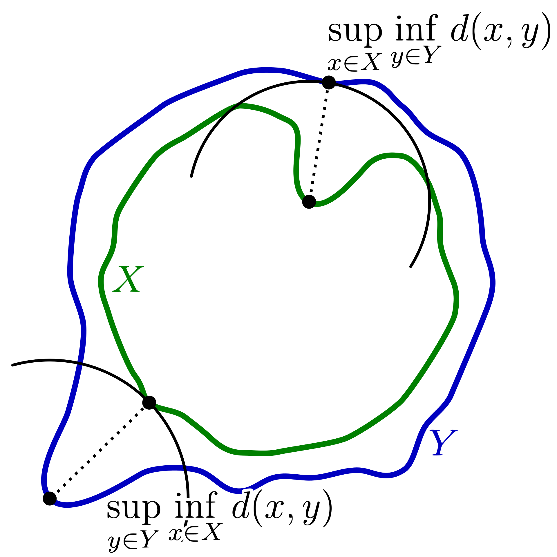
Hausdorff distance
Suppose and are subsets of a metric space .
The Hausdorff distance is:
Here:
- smallest distance to
- smallest distance to
Therefore:
- within , how far away can you get from ?
- within , how far away can you get from ?
Gromov-Hausdorff distance
Suppose and are compact metric spaces and is some fixed compact metric space.
The Gromov-Hausdorff (GH) distance is:
where , are isometric embeddings of , into .
Notice that this definition is relative to .
Link to original
Theory - Dendrogram
Dendrogram
Persistent homology describes the clustering of point-cloud data.
The GH distance frequently serves as a pure math benchmark. Given finite sets of points , the distance is a measure of similarity of the shape of the point clouds and .
The GH distance cannot be computed efficiently (if at all), so other measures of similarity for point clouds are useful.
Desiderata for measures of point-cloud similarity:
- Quantifies topological and geometric features
- Distinguishes features from noise
- Is computable
- Recognizes when features are close in the GH metric
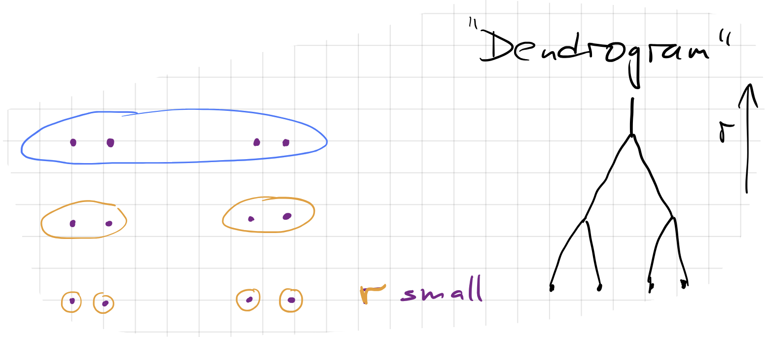
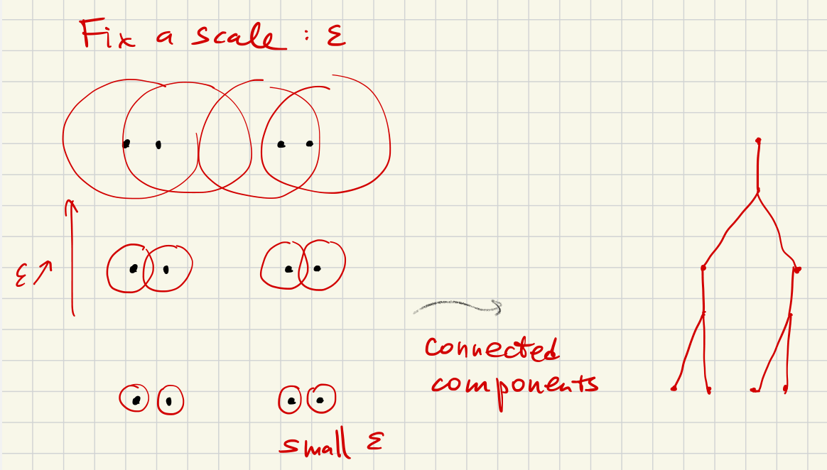
Suppose we have a finite set of points for a metric space .
Fix . Define a relation when .
Let be the transitive closure of . This is an equivalence relation (generated by ) which partitions into equivalence classes. Members of each equivalence class can be obtained from one another by a sequence of “hops” between points no more than apart.
Draw a tree diagram with a junction at each where distinct clusters are joined:
Link to original
Theory - Filtrations
Filtrations
Filtered simplicial complex
A filtered simplicial complex is a complex with a collection:
where each is a simplicial complex which is a subcomplex of .
(The vertices and simplices of a subcomplex must be vertices and simplices in the supercomplex.)
Filtered space
A filtered topological space is a collection of spaces indexed by with continuous maps:
and these maps satisfy a transitivity compatibility:
It is sometimes convenient, if a little ungainly, to consider a filtered simplicial complex as a filtered space where is a simplicial subcomplex of whenever . Such a filtered space changes only at discrete values of .
Link to original
Illustration
Čech complex as filtered complex
Link to originalČech complex as filtered complex
Let be a finite set of points in a metric space .
Recall that the Čech complex of , written for , is the nerve complex of the collection of open balls .
In other words, is the complex with vertices the points of , and -simplices the subsets with points whose -balls have nonempty mutual intersection.
This is a filtered complex because whenever . Once in, always in, for a simplex.
Theory - Vietoris-Rips complex
Vietoris-Rips complex
Vietoris-Rips complex
Let be a finite set of points in a metric space .
The Vietoris-Rips complex is the complex whose vertices are the points , and whose -simplices are those subsets with points all of which are pairwise less than apart:
The VR complex is a filtered space (filtered complex) because:
Notice that the VR complex and the Čech complex include the same 1-simplices: a simplex is in the VR complex if , and in the Čech complex if . These conditions are equivalent, at least in .
Pairwise vs. mutual intersection
- The VR complex includes simplices for points which pairwise intersect.
- The Čech complex includes simplices for points which mutually intersect.
For example:
The three blue circles all intersect pairwise, so is in the VR complex, but they don’t mutually intersect so this simplex is not in the Čech complex.
On the other hand, the four green circles do not intersect pairwise. The VR complex and the Čech complex are the same in this case.
VR complex computability
Since the VR complex depends only on the data of pairwise distances between points, it is very easy to compute.
Čech and VR containments
For any point cloud , we have:
- inclusion as subcomplex
- inclusion as subcomplex
The first is true because any mutual intersection implies the pairwise intersections.
The second is true because any pairwise intersection of balls implies that the balls extend to cover other centers. So the centers of all points are in the -balls of each of the others, thus the centers are in the mutual intersection.
Link to original
Theory - Persistent homology, barcodes
Persistent homology, barcodes
Persistent homology
Let be a filtered simplicial complex.
Fix . For any , define:
Whenever there is a map and this induces linear maps on homology:
These satisfy .
The persistent homology of is the collection of vector spaces and linear maps .
Persistent homology is defined for any filtered simplicial complex. For example, we can take persistent homology of the Čech complex or of the Vietoris-Rips complex.
Persistent VR homology - Structure Theorem
Let for be the persistent homology of the VR complex of a point cloud .
Fix . Then has a canonical decomposition as a direct sum of persistence intervals:
Link to originalPersistence interval
For any with and , define:
with (linear) filtration maps given by when .
Illustration
Illustration - barcode and persistence diagrams
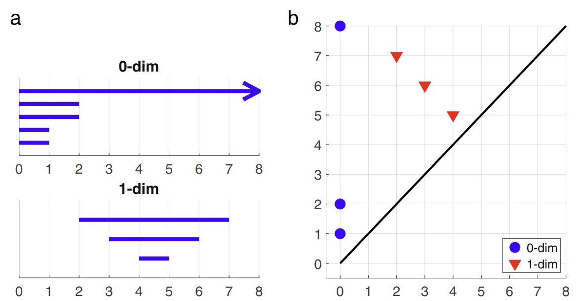
Barcode diagram:
- Each receives a horizontal bar starting at , ending at .
- Bar colored according to degree in
Persistence diagram:
Link to original
- Each receives a dot placed at
- Horizontal ‘birth’ axis, vertical ‘death’ axis
- Dots colored according to degree in
Point cloud - square
Link to originalPoint cloud: square
Basis:
Decomposition:
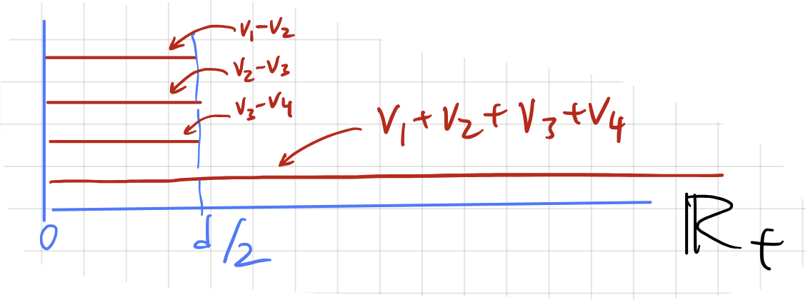
Filtered complex
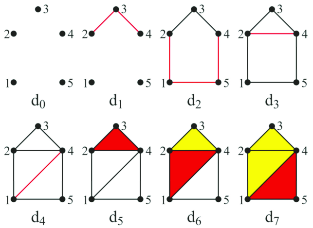
Link to originalFiltered complex
Abstract filtration:
Barcode and persistence diagram:
Theory - Barcode basis
Barcode basis
We would like to understand the direct sum decompositions like the one in the example of the point cloud square:
Understanding such a decomposition amounts to determining a basis of homology classes that have lifespans described by the persistence intervals.
We have:
A basis for is the equivalence class of all vectors in which are not in the span . For example, or or .
Barcode diagram for :
Now consider . Cycles in are generated by 1-simplices which are sets of two points that are apart.
Consider again the square point cloud:
For , we have .
For , we have .
For , we have 4 additional 2-simplices (all combinations of 3 points).
The square will the boundary of the difference of two of the 2-simplices (complementary triangles), so the homology class of the square vanishes when reaches .
Barcode diagram for :
Thus:
Link to original
Stability
Theory - Bottleneck distance
Bottleneck distance
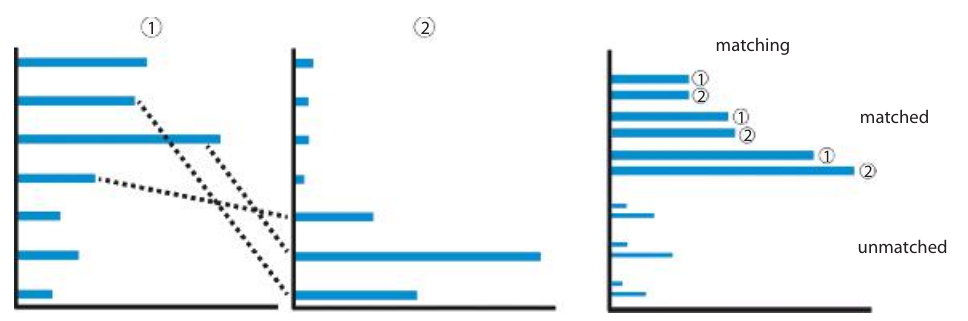
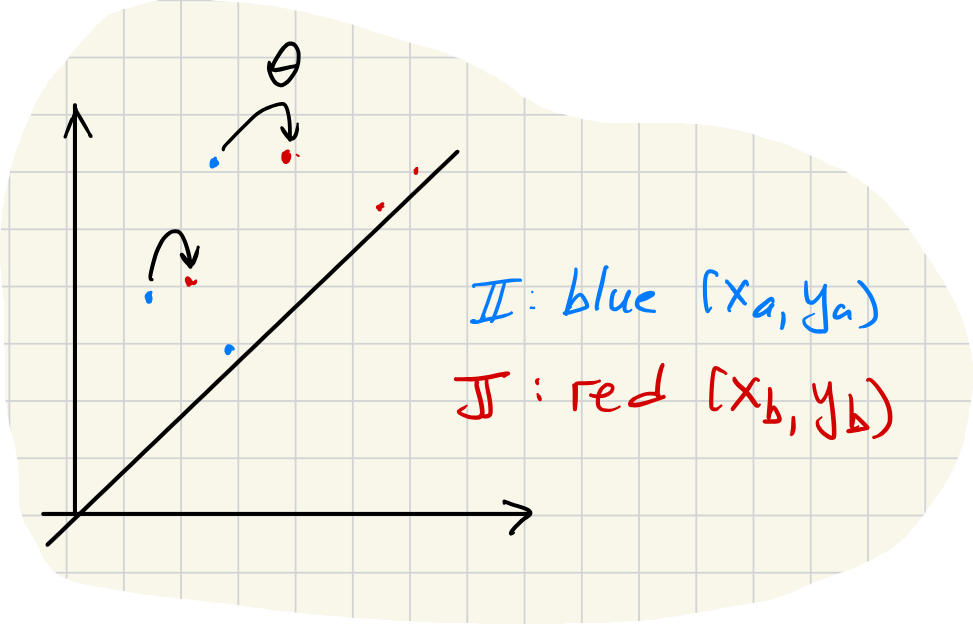
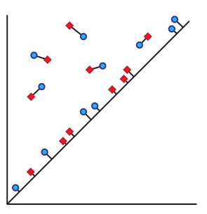
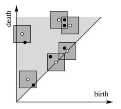
The bottleneck distance is a metric on barcode diagrams. The bars in one barcode are matched against the bars in the other. The distance between barcodes is the worst discrepancy between bars in the optimal matching.
Suppose we are given two barcode diagrams. These are two finite collections of intervals:
Now define the -distance between two intervals by:
Also, define:
This is the -distance to the nearest point-interval .
Now, suppose we are given subsets and along with a choice of bijection . Define the penalty of to be:
Bottleneck distance
The bottleneck distance from to is:
Bars far from the diagonal are matched to the closest bars (using the -norm whose unit balls are squares). Bars near the diagonal can be matched to the closest diagonal point. The distance to the closest point on the diagonal is .
Stability Theorem: Bottleneck Distance
Let and be two finite metric spaces. Fix . Let be the barcode diagram for and let be the barcode diagram for . Then:
This theorem is a kind of “stability” result regarding barcode diagrams, since it says that when two data sets and are close together (measured using the ideal, if not computable, metric ), then the barcode diagrams are also close together. Barcode diagrams cannot jump apart without the data sets jumping apart.
For example, if is a “noisy” version of , then we expect to be small, and therefore the barcode diagrams should be close. Conversely, if barcode diagrams are far, the data sets differ by “more than noise.”
Link to original
Theory - Wasserstein metrics
Wasserstein metrics
The Wasserstein metrics generalize the bottleneck metric. Instead of taking the worst discrepancy between two bars in the best matching, it uses a -sum of the discrepancies of all bars in the best matching.
First define the -penalty for a partial matching as follows:
Then we minimize the penalty (find the best matching):
Link to originalRemark
We can recast the -penalty in a more uniform symbolism by supplementing or with empty bars so that each has the same number of “bars,” and recalling the convention that . Then we have:
Multi-dimensional persistent homology
Theory - Several parameters
Several parameters
Thus far the persistent homology we have considered is derived from filtered spaces/complexes with a single filtration parameter :
It is possible to combine two types of filtration in a single structure having inclusion maps of each type.
Unfortunately there is no “structure theorem” for persistent homology with more than one parameter. This is basically because the structure theorem proof in one parameter involves homology with coefficients, while with parameters it involves homology with coefficients.
Link to original
Illustration
Filtering also by density
Link to originalFiltering also by density
Let us add a density filtration to . Fix and define by:
Now the points in , and the -complex itself, can be filtered by a density minimum:
This bi-filtered complex determines a 2-parameter persistence module:
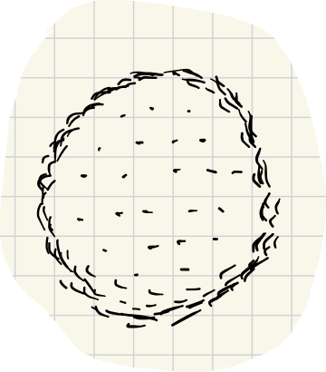
For large , only points very close to distinct neighbors are included. As decreases, more points are brought in.
With data like this, the filtration (for middling values) removes points inside the disk because they are too sparse.
Filtering also by distance to a subspace
Link to originalFiltering also by distance to a subspace
Suppose is an embedded -dimensional subspace of the background space that contains the data:.
Let measure the distance from data points to the image of .
Define . This gives a filtration in terms of the parameter . This filtration could be useful if the complete data set is too big to process all at once. The filtration allows one to process the data in layers.
These filtrations determine inclusions of complexes. For fixed and , we have:
Upon applying homology, for , we have:
And for fixed and , we have:
Upon applying homology, we have:
Finally, these induced maps should commute with each other:
Theory - Zig-zag persistent homology
Zig-zag persistent homology
Filtrations can be modified in another way by adding intermediate linking sets. Instead of the usual filtered space like this:
We have a “zig-zag” filtered space like this:
In general, each arrow is allowed to go either direction. The induced map on homology will follow the same pattern.
Link to original
Illustration
Morse layers
Link to originalMorse layers
An application of zig-zag filtration arises by dividing the entire space into small layers for which the homology is easier to compute. For example, with a Morse function , we have this zig-zag filtration:
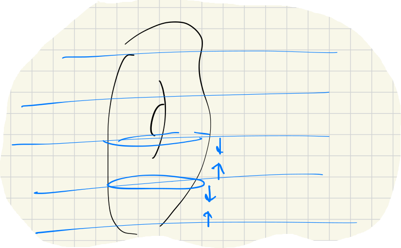
Repeated samples
Link to originalRepeated samples
Suppose some data is sampled repeatedly and data sets are generated in a sequence:
Then we can form a zig-zag filtration by:
Mapper algorithm
Theory - Clustering and Reeb graph
Clustering and Reeb graph
The mapper algorithm was introduced by Singh-Mémoli-Carlsson in 2007.
Recall the dendrogram (clustering) algorithm:
Given a fixed , two points are considered equivalent if there is a sequence of points
and the distance between successive points is much less than .
Now consider connected components (“clusters”) for each fixed . The clustering algorithm computes this and the calculation is essential the same as persistent homology for .
Link to originalReeb graph
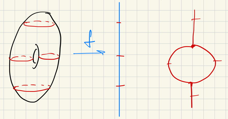
Given a Morse function on a manifold , the Reeb graph is formed by the equivalence relation:
Two points are equivalent if:
- AND
- are in the same connected component of
Mapper algorithm
Mapper algorithm
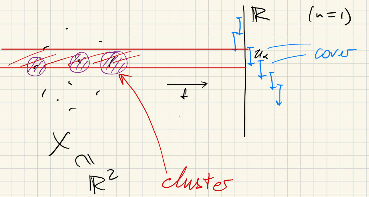
Let us be given:
- A finite metric space
- I.e. a finite collection of points with distances between them; usually
- A “filter function”
- A finite cover of in
- Typically a collection of boxes in
Proceed as follows:
(1) Consider the clustering of each :
- Choose and consider clusters at this scale .
- Write for the clusters, so
(2) Form a discrete version of the Reeb graph:
- Vertices: clusters
- Edges: when and overlap
- Color the vertices according to values of (on average):
Link to original
Illustration
Simple cover
Link to originalSimple cover
Suppose and suppose is just the interval containing the entire .
In this case Mapper produces a graph with no edges. Its vertices correspond to clusters of .
2-Component cover
Link to original2-Component cover
Suppose and suppose is the pair and . Mind the gap .
Vertices in the Mapper graph are -clusters of and of . These clusters must be all disjoint. So there are no edges between the vertices.
If, however, the cover had been chosen to be and , there could be vertices between clusters in and clusters in .
Consider data points sampled around the unit circle. Let by . Suppose the image is covered by small overlapping intervals of equal length. Mapper recovers the topology of the circle:
If we had used a simple cover (single interval), the Mapper graph would have no edges and thus would not express the circle’s topology.
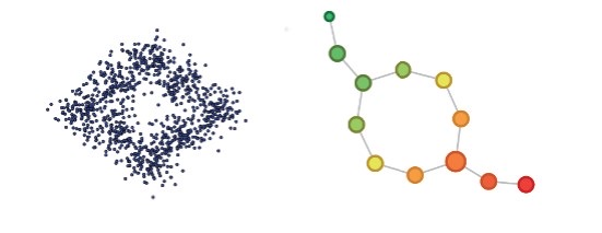
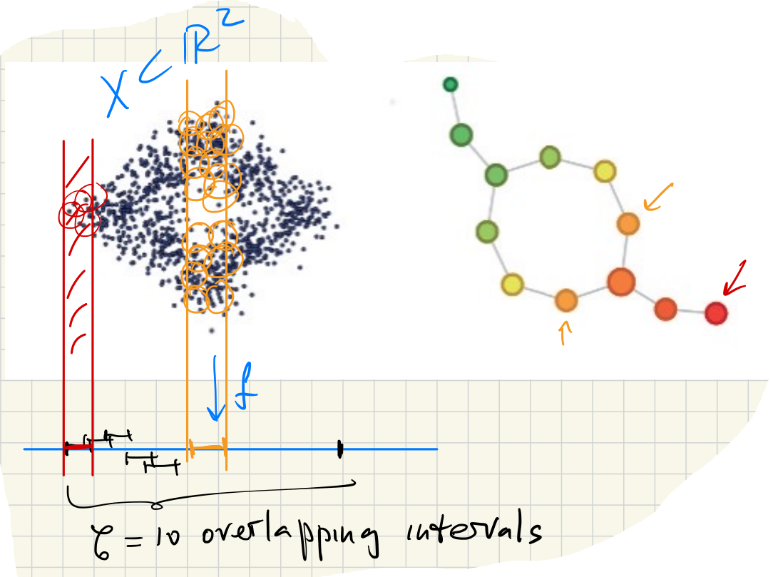
Illustration - Mapper figures from the literature
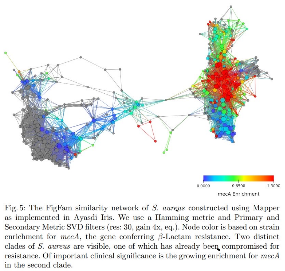
(Rabadan-Blumberg 2020)
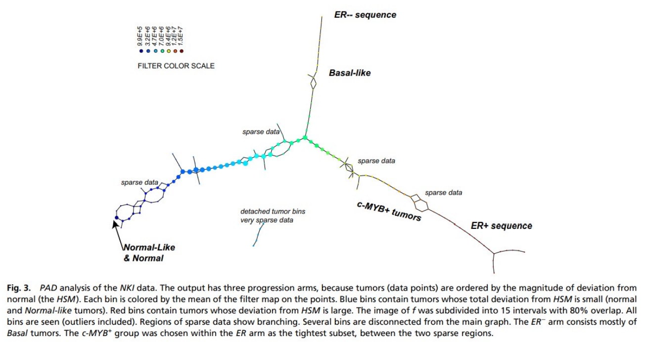
Link to original(Nikolau-Levine 2011)