Chapter 01 - First-Order Equations

What are differential equations?

Examples of differential equations

Examples of differential equations

The next examples illustrate what some important differential equations look like. Some other matters come up too, for example that solutions to differential equations are functions (not numbers), and that a single equation can have many solutions.

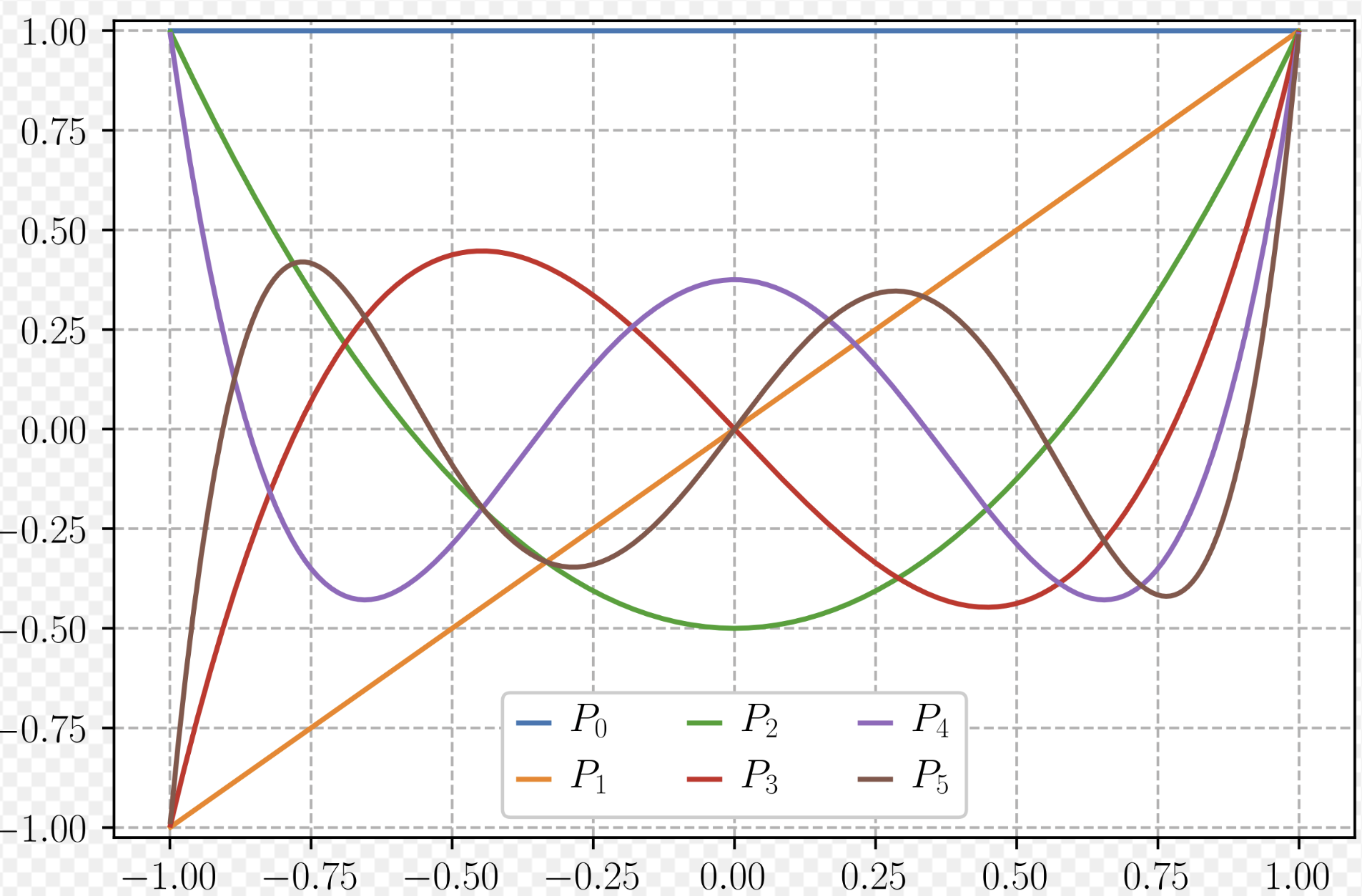
Legendre’s equation:

$$(1-x^2)\frac{d^{2}y}{d{x}^2}-2x\frac{dy}{dx}+n(n+1)y=0.$$

The solution to this equation is a polynomial $y=P_n(x)$ for each $n$. The first few polynomials are:

$n$	$P_n(x)$
0	1
1	$x$
2	$\frac{1}{2}(3x^2-1)$
3	$\frac{1}{2}(5x^3-3x)$

These polynomials have many useful properties. Their most important property is “orthogonality”:

$${\int }_{-1}^{+1}{P}_n(x)P_m(x)dx=0\text{ unless }n=m.$$

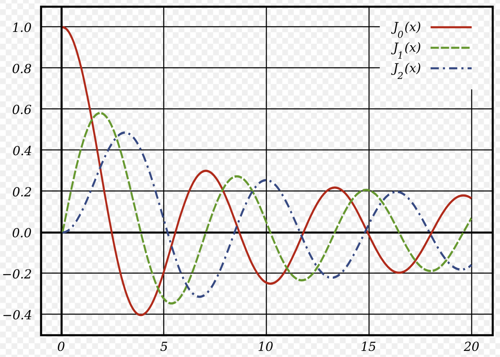
Bessel’s equation:

$$x^2\frac{d^{2}y}{d{x}^2}+x\frac{dy}{dx}+(x^2-{\alpha }^2)y=0.$$

Solutions to this equation are used to study heat conduction and waves (electromagnetic or quantum wavefunctions).

Airy’s equation:

$$\frac{d^{2}y}{d{x}^2}-xy=0.$$

The solution to Airy’s equation arises in quantum mechanics, optics, and probability.

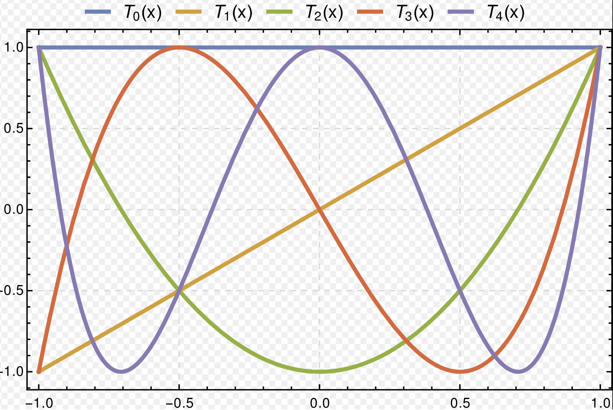
Chebyshev’s equation:

$$(1-x^2)y^{\prime \prime }-x{y}^{\prime }+p^{2}y=0.$$

Solutions to this equation give polynomials $T_n(x)$ and $U_n(x)$ that describe the higher sum rules of trig functions:

$$\begin{array}{rl}\cos (n\theta )& =T_n(\cos (\theta ))\\ \sin (n\theta )& =\sin (\theta )U_{n-1}(\cos (\theta )).\end{array}$$

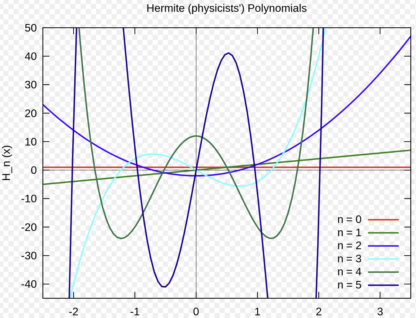
Hermite’s equation:

$$y^{\prime \prime }-2x{y}^{\prime }+2py=0.$$

Solutions to this equation are used in quantum mechanics, signal processing, numerical analysis, and probability.

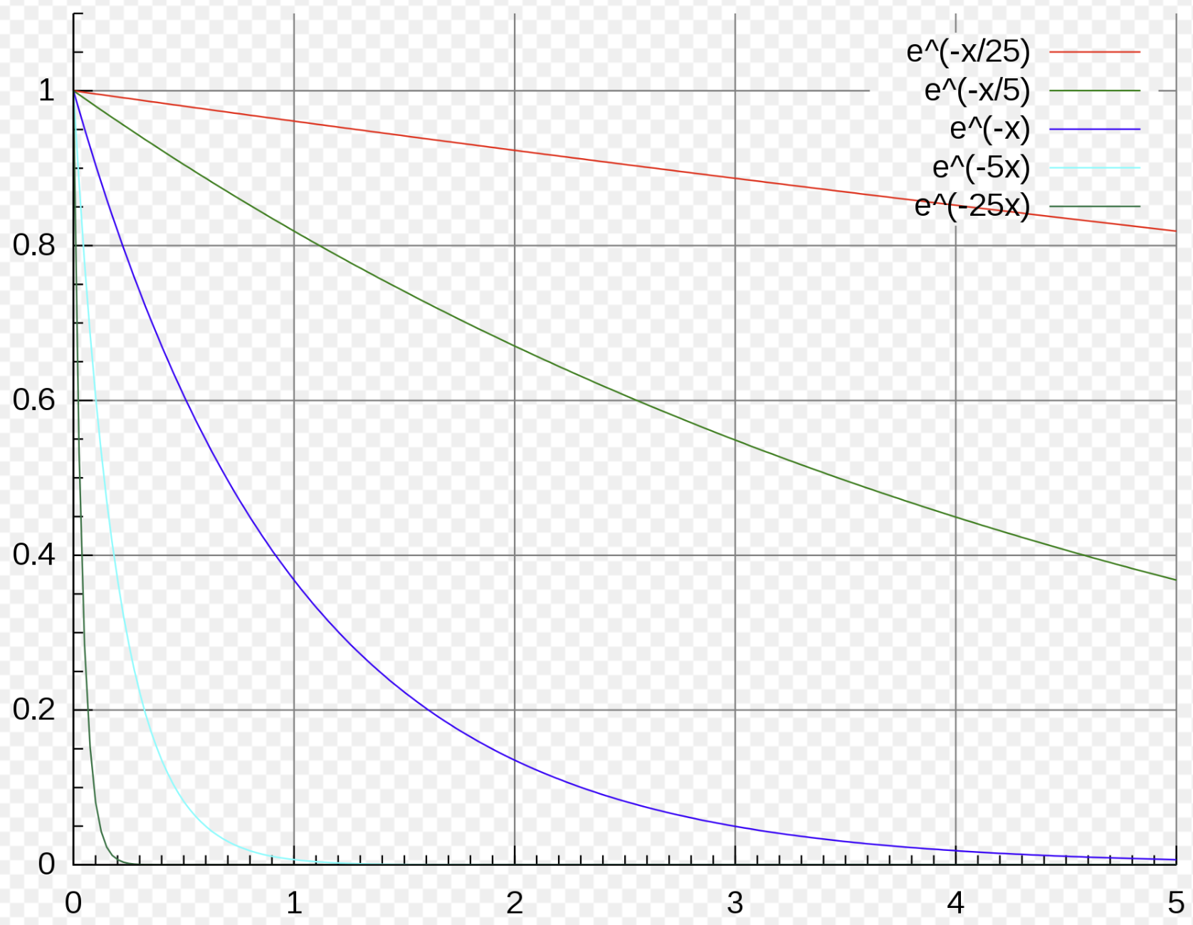
Exponential decay:

$$\frac{dy}{dx}-ky=0.$$

This equation models countless physical processes.

Link to original

Concepts of differential equations

Concepts of differential equations

What we typically mean by a “differential equation” is a function $F$ of, say, $n+2$ variables, that is given by some algebraic expression (possibly involving trig or exponential functions as well). A solution to the equation is a function $y(x)$ with the property that:

$$F\left(x,y(x),y^{\prime }(x),y^{\prime \prime }(x),\dots ,y^{(n)}(x)\right)=0$$

for all $x$. The order $n$ of the differential equation is the order of the highest derivative that appears in the expression for $F$.

A differential equation is called explicit when it can be written with the highest derivative isolated, on the other side:

$$F(x,y,y^{\prime },\dots ,y^{(n-1)})=y^{(n)}.$$

Sometimes a differential equation is “solved” by finding an equation relating $y$ and $x$ which cannot be solved explicitly for $y$ in terms of $x$. In this situation, a (connected) set of points $(x,y)$ satisfying the solution equation is called an integral curve of the differential equation.

Ordinary differential equations involve only ordinary derivatives, while partial differential equations involve partial derivatives.

Usually we assume that $F$ is a familiar kind of function that is constructed using algebraic operations (possibly with trig or exponential functions) applied to the arguments.

There is a fundamental distinction between linear and nonlinear differential equations. A linear differential operator is a linear function taking functions to functions. For example:

$$\left(\frac{d^2}{d{x}^2}-x\right):y(x)⟼\frac{d^{2}y}{d{x}^2}-xy.$$ Link to original

Question

01

Linear operator

Show that the example differential operator above satisfies the linearity equation for two given functions $y_1(x)$ and $y_2(x)$. Let $F=\left(\frac{d^2}{d{x}^2}-x\right)$; show that:

$$F(a{y}_1+b{y}_2)=aF(y_1)+bF(y_2).$$

Link to original

Concepts of differential equations (part 2)

Linear differential equations are defined as those corresponding to a linear differential operator. (By applying the operator to $y$ and setting the result equal to some function.) Roughly speaking, this means they are equations in which $y,y^{\prime },y^{\prime \prime },\dots$ can appear only to the first power.

Link to original

First-order equations

Introduction

A first-order (explicit) ODE looks like this:

$$\frac{dy}{dx}=f(x,y)$$

for some function $f$.

Many techniques for solving first-order ODEs come from reverse-engineering results of calculus. In this respect, solving ODEs analytically is like taking integrals (finding antiderivatives) analytically. In fact, antidifferentiation is itself one of the techniques: when $f(x,y)$ does not depend on $y$, both sides of the equation above can be integrated to find $y(x)$. More advanced methods like the product rule or $u$-substitution yield more sophisticated techniques for ODEs.

Link to original

Direct integration

Direct integration

A differential equation of the form:

$$\frac{dy}{dx}=f(x)$$

has a set of solutions given by $y=F(x)+c$ where $c$ is any constant and $F$ is an antiderivative of $f$, meaning $F^{\prime }=f$.

This kind of differential equation is really a part of basic calculus. A few things to emphasize en route to more complicated ODEs:

• There is a family of solutions parametrized by some constant $c$. (This will become a pattern.)
• This family is a complete set: there are no other solutions. (Why not?)
• A particular solution is determined (selected from this family) by a choice of initial condition, which consists of a point $(x_0,y_0)$ that should lie on the solution.
• Consider that the derivative value specifies the direction of travel. So the initial condition is a starting point, and $f(x)$ gives the data of which way to go, changing course along the route.

This technique can be applied in a series for simple ODEs of higher order. For example, the ODE

$$\frac{d^{2}y}{d{x}^2}=f(x)$$

is solved by taking two antiderivatives. Let ${\Phi }^{\prime }=F$ and $F^{\prime }=f$. Then we have a family of solutions that depends on two constants:

$$y(x)=\Phi (x)+c_{1}x+c_2.$$

To specify a particular solution, one provides two points $(x_1,y_1)$ and $(x_2,y_2)$ that should lie on the solution, and you can solve for $c_1$ and $c_2$ by evaluating $\Phi (x_1)$ and $\Phi (x_2)$.

Link to original

Question

01

Checking things

• For the first-order equation above, why must $F(x)+c$ give a complete set of solutions?
• For the second-order equation, explain how to obtain the formula $\Phi (x)+c_{1}x+c_2$.

Link to original

$★$ Question

02

Higher order

(Big Bonus question. Not for the faint of heart!)

• Can any two points $(x_0,y_0)$ and $(x_1,y_1)$ be chosen?
• Now iterate the process: consider $y^{(n)}=f(x)$ and solve using multiple consecutive integrations. Describe the family of solutions. What constraints are there on the set of points $(x_0,y_0),\dots ,(x_n,y_n)$ needed to specify a particular solution?

Link to original

Direct integration (part 2)

Instead of providing multiple points lying on the solution, one can choose a single value $x_1$, and then specify the values of the higher derivatives $y^{(i)}(x_1)=b_i$ using some numbers $b_0,\dots ,b_{n-1}$.

Link to original

Separable equations: substitution

Separable equations - substitution

Consider again the general form of an explicit first-order ODE:

$$\frac{dy}{dx}=f(x,y).$$

This ODE is called separable when $f(x,y)=g(x)h(y)$ for some product of functions of the separate variables, $g(x)$ and $h(y)$. It is solved by integrating separately in $x$ and in $y$, as we consider next.

Consider any function $a(y)$ with antiderivative $A(y)$, so $A^{\prime }=a$. The chain rule says:

$$\frac{d}{dx}A(y)=A^{\prime }(y)\frac{dy}{dx}=a(y)\frac{dy}{dx}.$$

Now let $a(y)=\frac{1}{h(y)}$. The differential equation

$$\frac{dy}{dx}=g(x)h(y)$$

is equivalent to the equation

$$a(y)\frac{dy}{dx}=g(x),$$

so we end up with

$$\frac{d}{dx}A(y)=g(x),$$

which is solved by integrating both sides in $x$ to obtain:

$$A(y)=G(x)+c,$$

where $G^{\prime }=g$ is an antiderivative of $g$ and $c$ is a constant of integration.

Think about this equation $A(y)=G(x)+c$. It equates the antiderivatives of $1/h(y)$ and $g(x)$ (up to a constant). It is an implicit definition of $y(x)$, because it may be virtually impossible to solve for $y$ here as a function of $x$. And, for the same reason as used for the ODE $y^{\prime }(x)=f(x)$ earlier, the family of implicit curves given by this equation (for various $c$) describes all possible solutions.

Many authors describe the solution method a little differently. Starting with

$$\frac{dy}{dx}=g(x)h(y),$$

write it as

$$\frac{dy}{h(y)}=g(x)dx$$

and “integrate” both sides, summing up the differentials:

$$\int \frac{1}{h(y)}dy=\int g(x)dx.$$

This yields

$$A(y)=G(x)+c$$

as before.

This method is easy to remember, and is acceptable to use on an exam or HW, but it is not really standard calculus procedure, since it relies on ambiguous rules about differentials. (Normally in calculus books differentials are considered purely mnemonic devices.)

Link to original

Example

Separable ODE

Separable ODE

Problem: Solve the equation $y^{\prime }=2xy$.
Solution: The given equation can be written

$$\frac{dy}{y}=2xdx.$$

Integrating both sides, obtain

$$\ln |y|=x^2+c.$$

Applying $e^{-}$ on both sides:

$$|y|=e^{x^2+c}.$$

Applying the exponent sum rule and writing $C=e^c$, we get

$$|y|=C{e}^{x^2}C>0.$$

Here $C>0$ because $e^c>0$ for any $c\in \mathbb{R}$. However, we can allow $C<0$ by removing the absolute values. So that family of functions is the same as this family:

$$y=C{e}^{x^2}C\in \mathbb{R}.$$

Note that the $C=0$ solution, $y=0$, is valid but isn’t generated by separation of variables because of the division by $y$ that was performed in the first step.

Link to original

Exercise

01

Tricky signs

Check and explain all absolute values and signs (including $C>0$) in the previous example.

Link to original

Example

Integral curves

Integral curves

Problem: Solve the separable ODE:

$$\frac{dy}{dx}=\frac{x^2}{1-y^2}.$$

Solution: Rewrite this as:

$$(1-y^2)dy=x^{2}dx$$

and integrate both sides to obtain:

$$y-\frac{y^3}{3}=\frac{x^3}{3}+c.$$

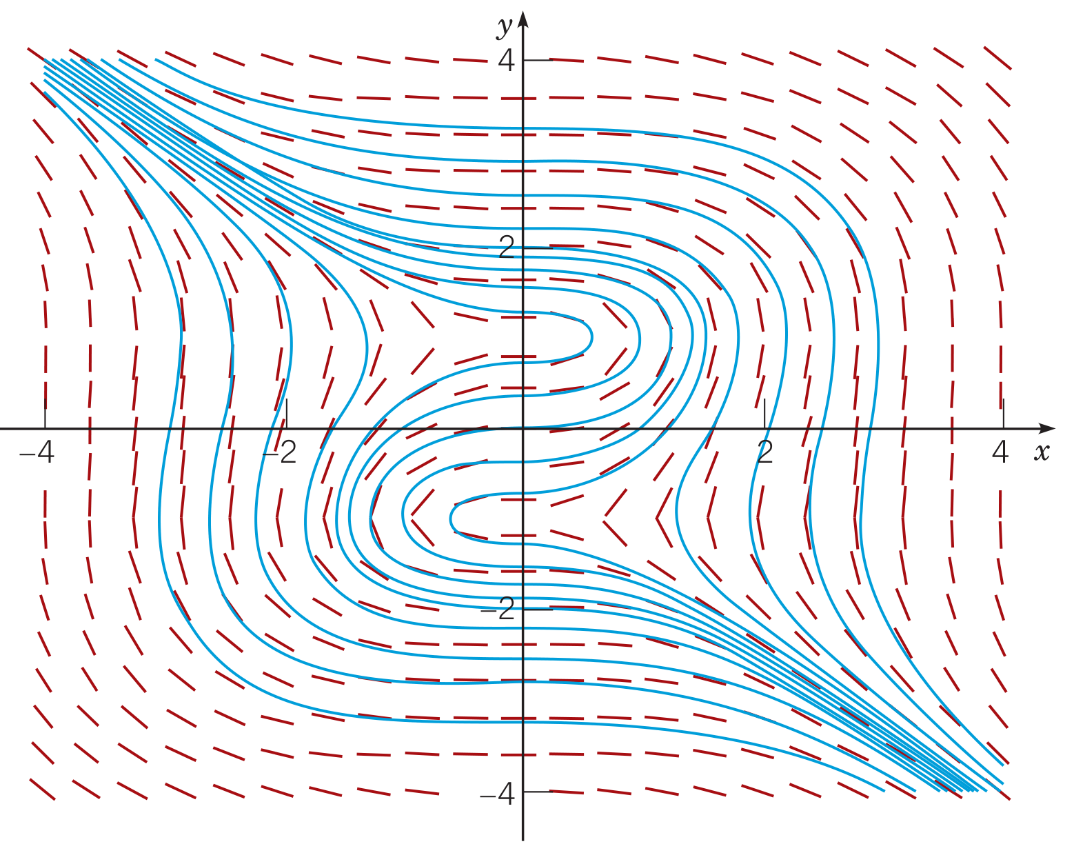
This equation specifies a family of integral curves. For the integral curves, we do not need to solve for $y$ in terms of $x$. Here is a depiction:

Link to original

Exercise

02

Separable equations: basics

Solve the equations:

• (a) $x^5{y}^{\prime }+y^5=0$
• (b) $x{y}^2-y^{\prime }{x}^2=0$

Link to original

Exercise

03

Separable equations: tricky trig

Solve the equation:

$$x{y}^{\prime }=(1-4x^2)\tan (y).$$

After finding the basic solution, check over the signs and absolute values of everything.

Link to original

Exercise

04

Particular solution

Find the particular solution to

$$\frac{y^{\prime }}{1+x^2}=\frac{x}{y}$$

which includes the point $(1,3)$.

Link to original

Linear equations: product rule

Linear equations - product rule

First-order linear equations have this general form:

$$y^{\prime }+a(x)y=b(x).$$

These equations are solved using the product rule together with an “integrating factor” $e^{\int a(x)dx}$. It works like this. Apply the product rule to $y\cdot e^{\int a(x)dx}$:

$$\begin{array}{rl}\frac{d}{dx}\left(y\cdot e^{\int a(x)dx}\right)& =y^{\prime }\cdot e^{\int a(x)dx}+y\cdot a(x)e^{\int a(x)dx}\\ & =e^{\int a(x)dx}\left(y^{\prime }+a(x)y\right).\end{array}$$

Now, multiply the original equation on both sides by $e^{\int a(x)dx}$ to find:

$$\frac{d}{dx}\left(y\cdot e^{\int a(x)dx}\right)=e^{\int a(x)dx}\left(y^{\prime }+a(x)y\right)=e^{\int a(x)dx}\cdot b(x).$$

Integrate both sides with respect to $x$:

$$y\cdot e^{\int a(x)dx}=\int e^{\int a(x)dx}\cdot b(x)dx+c,$$

which can be solved for $y$:

$$y=e^{-\int a(x)dx}\int e^{\int a(x)dx}\cdot b(x)dx+c{e}^{-\int a(x)dx}.$$ Link to original

Example

First-order linear

First-order linear

Problem: Solve the equation:

$$x^2{y}^{\prime }+xy=x^3.$$

Solution: First divide by $x^2$ to recover the standard format:

$$y^{\prime }+x^{-1}y=x.$$

Now the integrating factor we need is $e^{\int x^{-1}dx}=e^{\ln |x|}=|x|$. Multiply everything by this factor:

$$|x|y^{\prime }+\frac{|x|}{x}y=x|x|.$$

If $x>0$ everywhere, we can drop the absolute value signs obtaining $x{y}^{\prime }+y=x^2$. If $x<0$ everywhere, we would need to introduce minus signs (recall that $|x|=-x$ and $|x|/x=-1$ when $x<0$), obtaining $-x{y}^{\prime }-y=-x^2$; but this we can multiply by $-1$ and obtain the same equation, namely:

$$x{y}^{\prime }+y=x^2.$$

Let us solve this and come back later to consider the possibility of $x$ changing signs.

The sum on the left is the output of the product rule: ${\left(xy\right)}^{\prime }=x{y}^{\prime }+y$. Now integrate in $x$ to find a family of solutions:

$$\begin{array}{rl}xy& =\int x^{2}dx=\frac{1}{3}{x}^3+c,\\ y& =\frac{1}{3}{x}^2+\frac{c}{x}.\end{array}$$

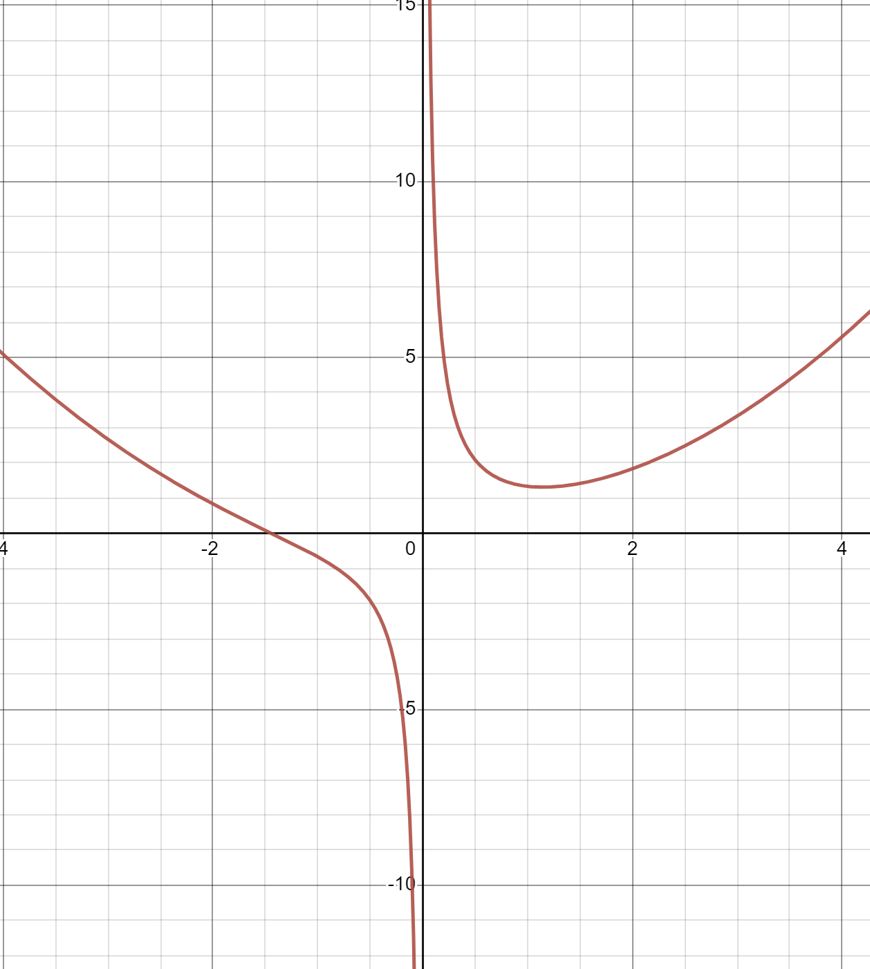
This family, for various values of $c\in \mathbb{R}$, is our proposed solution to the ODE.

Now reconsider the absolute values. Suppose $c>0$. If we take a solution curve with $x>0$, then the entire curve will satisfy $x>0$ because $y\to +\infty$ as $x\to 0^{+}$. Similarly, if we start with $x<0$, then $y\to -\infty$ as $x\to 0^{-}$. No solution crosses over $x=0$. Now if $c<0$ we can say the same thing but with $y\to -\infty$ and $y\to +\infty$, respectively, instead. Therefore our analysis using cases $x>0$ and $x<0$ is justified.

Link to original

Exercise

05

Linear equations: basics

Solve the following ODEs, giving a complete family of solutions:

• (a) $y^{\prime }+xy=x$,
• (b) $y^{\prime }+y\cot (x)=2x\csc (x)$.

Link to original

Exercise

06

Linear equation: particular solution

Find a particular solution of the following ODE which passes through the point $(0,0)$:

$$y^{\prime }-2xy=6x{e}^{x^2}.$$

Link to original

Exact equations: gradients

Exact equations - gradients

A final technique is based on more advanced calculus.

Recall the theorem of vector calculus:

Curl-free fields are gradients

Suppose $\mathbf{F}(x,y)$ is a vector field on ${\mathbb{R}}^2$ with zero curl: $\nabla \times \mathbf{F}=0$. (Assume the region is simply-connected.) Then there is a scalar field $f(x,y)$ whose gradient recovers the vector field: $\mathbf{F}=\nabla f$.

Writing out the components, this theorem says that if

$$\frac{\partial F_2}{\partial x}-\frac{\partial F_1}{\partial y}=0,$$

then there is a function $f$ satisfying

$$F_1=\frac{\partial f}{\partial x}\text{and}{F}_2=\frac{\partial f}{\partial y}.$$

Now, finally, let $\mathcal{C}$ be a level curve given by $f(x,y)=c$ for some $c$. Then $\nabla f$ is perpendicular to $\mathcal{C}$. This latter fact can be interpreted as a differential equation with $\mathcal{C}$ one of its integral curves, as we show next.

Let $y=y(x)$ be considered a function of $x$ whose graph is the curve $\mathcal{C}$. Then $\mathcal{C}$ may be described parametrically by $(x,y(x))$, and the tangent vector to this parametric curve is described parametrically by $(1,y^{\prime }(x))$. The condition $\nabla f\perp \mathcal{C}$ is equivalent to $\nabla f\cdot (1,y^{\prime })=0$, which when written out means:

$$\frac{\partial f}{\partial x}+\frac{\partial f}{\partial y}{y}^{\prime }=0.$$

Writing $M(x,y)=\frac{\partial f}{\partial x}$ and $N(x,y)=\frac{\partial f}{\partial y}$ and $y^{\prime }=\frac{dy}{dx}$, and multiplying through by $dx$, we obtain a form that is easier to remember:

$$M(x,y)dx+N(x,y)dy=0.$$

Here is a summary of our reasoning:

Exact equations

Suppose the differential equation written either in form (A):

$$M(x,y)dx+N(x,y)dy=0$$

or in form (B):

$$M(x,y)+N(x,y)\frac{dy}{dx}=0$$

satisfies $\frac{\partial M}{\partial y}=\frac{\partial N}{\partial x}$. Then it has a family of solutions given by the level curves $f(x,y)=c$, where $f$ is a function satisfying $\frac{\partial f}{\partial x}=M$ and $\frac{\partial f}{\partial y}=N$.

Algebraic summary

A more algebraic formulation of the same theory goes like this:

If $\frac{\partial M}{\partial y}=\frac{\partial N}{\partial x}$, then it is possible to find $f(x,y)$ such that $\frac{\partial f}{\partial x}=M$ and $\frac{\partial f}{\partial y}=N$. In this case the equation

$$M(x,y)+N(x,y)y^{\prime }=0$$

can be written

$$\frac{d}{dx}(f(x,y(x)))=0$$

using the chain rule, and this has as solutions the family of integral curves defined implicitly with constants $c\in \mathbb{R}$:

$$f(x,y(x))=c.$$

Link to original

Example

Solving an exact equation

Solving an exact equation

Problem: Solve the ODE:

$$e^{y}dx+(x{e}^y+2y)dy=0.$$

Solution: First we check that $\frac{\partial M}{\partial y}=\frac{\partial N}{\partial x}$:

$$\begin{array}{rl}\frac{\partial M}{\partial y}& =e^y\\ \frac{\partial N}{\partial x}& =e^y+0=e^y.\end{array}$$

Now we seek $f(x,y)$ with $\frac{\partial f}{\partial x}=M=e^y$ and $\frac{\partial f}{\partial y}=N=(x{e}^y+2y)$. First integrate $e^y$ in $x$:

$$f(x,y)=\int e^{y}dx=x{e}^y+g(y)$$

where the “constant” can be any function of $y$. Now $\frac{\partial f}{\partial y}=x{e}^y+g^{\prime }(y)=x{e}^y+2y$, so $g^{\prime }(y)=2y$ and $g(y)=y^2+c$. Therefore our solution family of integral curves is given by:

$$x{e}^y+y^2=c$$

for $c\in \mathbb{R}$.

Link to original

Exercise

07

Checking exactness

Which of the following ODEs are exact?

• (a) $(\sin x+\tan y+1)dx+\cos x{\sec }^{2}ydy=0$
• (b) $(y-x^3)dx+(x+y^3)dy=0$
• (c) $(2x{y}^4+\sin y)dx+(4x^2{y}^3+x\cos y)dy=0$
• (d) $3x^2(1+\ln y)dx+\left(\frac{x^3}{y}-2y\right)dy=0$

Link to original

Exercise

08

Solving an exact equation

Show that the ODE is exact, and solve it:

$$\left(x+\frac{2}{y}\right)dy+ydx=0.$$

Link to original

Transformation and reduction

Introduction

So far we have seen how to solve differential equations by direct integration, by separation of variables, by integrating factors: conversion to a product (linear equations), and by gradients (exact equations).

Many differential equations do not immediately appear to have the standard form to which these methods are applicable, but in fact these methods can be applied after performing a transformation. The possibility of some of these transformations can be checked systematically, but for others we rely on an art – not a mechanical science – of finding an appropriate substitution. This art is based on experience and honed by practice.

Link to original

Homogeneous equations: conversion to separable

Homogeneous equations - conversion to separable

Homogeneous functions
A function is homogeneous when the input variable appears everywhere in the same degree. More precisely and technically, $f(x)$ is homogeneous when $f(tx)=t^{\alpha }f(x)$ for some $\alpha \in \mathbb{R}$. Similarly $g(x,y)$ is homogeneous when $g(tx,ty)=t^{\alpha }g(x,y)$ for some $\alpha \in \mathbb{R}$. (Likewise for more variables.) In this situation $\alpha$ is called the degree of homogeneity.

In other words, a function is homogeneous when the action of scaling the inputs simultaneously can be factored out to an action of scaling the output.

For example, these functions are homogeneous:

$$x^2+xy,\sin (x/y),\sqrt{x^2+y^2}$$

whereas these are not:

$$x^2+x,\sin (xy),x\sqrt{1-y^2}.$$

Homogeneous differential equations
Now, suppose we have a differential equation in the form:

$$\frac{dy}{dx}=\frac{M(x,y)}{N(x,y)},$$

where $M$ and $N$ are homogeneous functions of the same degree. Then the change of variables $z=y/x$ (by substituting $y=zx$) will convert the quotient on the right to a function of $z$ alone, and the equation as a whole to a separable equation, which we can solve for $z$ and at the end the solution can be converted to an expression in $y$ by substituting back $z=y/x$.

Homogeneous substitution

Suppose $M(x,y)$ and $N(x,y)$ are homogeneous of the same degree $\alpha$. Then $M(x,y)/N(x,y)$ depends only on the ratio $z=y/x$:

$$\frac{M(x,y)}{N(x,y)}=\frac{M(x,zx)}{N(x,zx)}=\frac{x^{\alpha }M(1,z)}{x^{\alpha }N(1,z)}=\frac{M(1,z)}{N(1,z)}=:F(z).$$

Separability then occurs because:

$$\frac{d}{dx}y=\frac{d}{dx}(zx)=\frac{dz}{dx}x+z,$$

so the equation $\frac{dy}{dx}=F(z)$ is equivalent to

$$\frac{dz}{F(z)-z}=\frac{dx}{x},$$

and the general solution is the family of curves given by:

$$\int \frac{dz}{F(z)-z}=\ln |x|+c.$$

Alternate format
The differential equation

$$M(x,y)dx+N(x,y)dy=0$$

is homogeneous if $M(x,y)$ and $N(x,y)$ are both homogeneous of the same degree. It can be transformed with the same substitution $z=y/x$ and the result is separable.

Link to original

Question

01

Homogeneous?

Is $x{y}^{\prime }=y+2x{e}^{-y/x}$ a homogeneous differential equation?

Link to original

Example

Homogeneous equation

Homogeneous equation

Consider the differential equation $x{y}^{\prime }=2x+3y$. Assuming $x\ne 0$, this is equivalent to the homogeneous equation $\frac{dy}{dx}=\frac{2x+3y}{x}$. Define $z=y/x$, and we find:

$$x\frac{dz}{dx}+z=2+3z\text{and so}\frac{dz}{1+z}=\frac{2}{x}dx.$$

The solution is therefore $\ln |1+z|=2\ln |x|+c$, or $1+z=C{x}^2$ for any $C\in \mathbb{R}$, i.e. $y=C{x}^3-x$ .

Link to original

Example

See an example in “Families of integral curves” below, where we solve the homogeneous equation $\frac{dy}{dx}=\frac{y^2-x^2}{2xy}$.

Exercise

01

Homogeneous equations

For the following differential equations, show that they are homogeneous, and then solve them by substitution and separation:

• (a) $(x^2-2y^2)dx+xydy=0$
• (b) $x^2{y}^{\prime }=3(x^2+y^2)\cdot {\tan }^{-1}(y/x)+xy$
• (c) $x{y}^{\prime }=\sqrt{x^2+y^2}$

Link to original

Homogeneous equations - conversion to separable (part 2)

Linear quotients: almost homogeneous
Suppose we are given a differential equation

$$\frac{dy}{dx}=\frac{a_{1}x+b_{1}y+c_1}{a_{2}x+b_{2}y+c_2}.$$

This equation is not homogeneous, but it is easily converted to a homogeneous equation by a change of variables. Find $h,k$ that solve the system:

$$\begin{array}{rl}{a}_{1}h+b_{1}k& =-c_1\\ a_{2}h+b_{2}k& =-c_2.\end{array}$$

Then by plugging in $x=u+h$ and $y=v+k$, the quotient on the right side is transformed to a quotient of homogeneous functions in $u$ and $v$:

$$\frac{dy}{dx}=\frac{a_{1}u+b_{1}v}{a_{2}u+b_{2}v}$$

The left side transforms as desired:

$$\frac{dy}{dx}=\frac{dy}{du}\cdot \frac{du}{dx}=\frac{dv}{du}\cdot 1=\frac{dv}{du}.$$ Link to original

Question

02

Transform linear quotient to homogeneous

Transform this equation to a homogeneous equation:

$$\frac{dy}{dx}=\frac{x+y+4}{x-y-6}.$$

Link to original

Integrating factors: conversion to exact

Integrating factors - conversion to exact

Sometimes an equation

$$M(x,y)dx+N(x,y)dy=0$$

is not exact, but there is a function $\mu (x,y)$ which when multiplied through the equation gives an exact equation:

$$\mu Mdx+\mu Ndy=0.$$ Link to original

Question

03

Integrating factor

Check that $x{y}^2$ is an integrating factor for $(2y-6x)dx+(3x-4x^2{y}^{-1})dy=0$.

Link to original

Integrating factors - conversion to exact (part 2)

How can we find such a function $\mu (x,y)$? There is no recipe that can find all possibilities for $\mu (x,y)$. However, if there is a $\mu$ that works and is a function of either $x$ or $y$ alone, then there is a recipe. Here it is:

Integrating factors: single variable

• Check $x$: if the function $g(x)=\frac{1}{N}(M_y-N_x)$ depends on $x$ alone, we can use $\mu (x)=e^{\int g(x)dx}$.
• Check $y$: if the function $h(y)=-\frac{1}{M}(M_y-N_x)$ depends on $y$ alone, we can use $\mu (y)=e^{\int h(y)dy}$.

Link to original

Exercise

02

Method of integrating factors

Show that if the function $g(x)=\frac{1}{N}(M_y-N_x)$ depends on $x$ alone, we can use $\mu (x)=e^{\int g(x)dx}$ as an integrating factor and the resulting differential equation becomes exact.

Link to original

Example

Integrating factor - converting to exact

Integrating factor: converting to exact

Consider the differential equation $(2x^2+y)dx+(x^{2}y-x)dy=0$. This is not exact because $M_y=1$ while $N_x=2xy-1$. However, $\frac{1}{N}(M_y-N_x)=-2/x=:g(x)$ is a function of $x$ alone. Therefore we can use $\mu (x)=e^{\int gdx}=x^{-2}$ as an integrating factor. Multiplying through by $x^{-2}$ produces the equation $(2+y{x}^{-2})dx+(y-x^{-1})dy=0$, which is exact because now $M_y=N_x=x^{-2}$.

Link to original

Exercise

03

Integrating factor: converting to exact

Convert the following to exact equations by finding and applying integrating factors.

• (a) $(x^4-x+y)dx-xdy=0$
• (b) $(2y^2+2y+4x^2)dx+(2xy+x)dy=0$

Link to original

Reduction of order

Reduction of order

Some second-order ODEs can be reduced to first-order ODEs by substituting $y^{\prime }=p$. This works when the equation $F(x,y,y^{\prime },y^{\prime \prime })$ is missing either $x$ or $y$.

If the equation is missing $y$, so the ODE is actually given by $F(x,y^{\prime },y^{\prime \prime })=0$, then we substitute $y^{\prime }=p$ and $y^{\prime \prime }=p^{\prime }$, and try to solve the equation $F(x,p,p^{\prime })=0$ as any other first-order equation. Afterwards we can solve for $y$ by integrating $p$ (provided we have an explicit solution for $p(x)$).

If the equation is missing $x$, so the ODE is actually given by $F(y,y^{\prime },y^{\prime \prime })=0$, then we substitute $y^{\prime }=p$ as before, but now we let $p=p(y)$ depend on $y$, and so $y^{\prime \prime }=p^{\prime }(y)p$ by the chain rule:

$$y^{\prime \prime }=\frac{dp}{dx}=\frac{dp}{dy}\frac{dy}{dx}=p^{\prime }(y)p.$$

We therefore try to solve the equation $F(y,p,p^{\prime }p)$ as any other first-order equation.

Link to original

Question

04

Reduction of order

Reduce the order of the following two differential equations. (No need to solve them.)

• (a) $x{y}^{\prime \prime }-y^{\prime }=3x^2$
• (b) $y{y}^{\prime \prime }=(y^{\prime }{)}^2$

Link to original

Example

Reduction of order

Reduction of order

Consider $x^2{y}^{\prime \prime }=(y^{\prime }{)}^2$. This equation is missing $y$ so we can reduce it to a first-order equation by letting $y^{\prime }=p$ and $y^{\prime \prime }=p^{\prime }$. The equation becomes $x^2{p}^{\prime }=p^2$ which is separable. The solution is $p=\frac{x}{1+c_{1}x}$, and this implies $y=\frac{x}{c_1}-\frac{1}{c_1^2}\ln (1+c_{1}x)+c_2$. (Integrating $p(x)=y^{\prime }(x)$ to obtain $y(x)$.)

Consider $y^{\prime \prime }+k^{2}y=0$. This equation is missing $x$ so we can reduce it to a first-order equation by letting $y^{\prime }=p$ and $y^{\prime \prime }=p^{\prime }p$. The equation becomes $p\frac{dp}{dy}+k^{2}y=0$ which is separable. The solution is $p(y)=\frac{dy}{dx}=\pm k\sqrt{c_1-y^2}$. This is a new differential equation which is also separable. Its general solution is $y=\sqrt{c_1}\sin (\pm kx+c_2)$.

Link to original

Ad hoc transformations

Ad hoc transformations

Bernoulli equations
The Bernoulli equations look like linear equations but with an extra factor of $y^n$:

$$\frac{dy}{dx}+a(x)y=b(x)y^n.$$

If we substitute $v=y^{1-n}$, a Bernoulli equation becomes a linear equation.

Link to original

Exercise

04

Bernoulli substitution

Show that substituting $v=y^{1-n}$ does indeed convert the Bernoulli equation to a linear equation.

Link to original

Exercise

05

Solving Bernoulli equations

Solve the Bernoulli equation $ydx+xdy=x{y}^{2}dx$.

Link to original

Ad hoc transformations (part 2)

Linear substitutions
If in the general form of an explicit first-order equation $y^{\prime }=f(x,y)$ the items $x$ and $y$ only occur together in a linear combination, so it really takes the form $y^{\prime }=f(ax+by)$, then we can change variables using $z=ax+by$ and then separate variables. First convert $y^{\prime }$:

$$\frac{dy}{dx}=\frac{d}{dx}\left(\frac{z(x)-ax}{b}\right)=\frac{z^{\prime }(x)-a}{b},$$

then the equation $y^{\prime }=f(ax+by)=f(z)$ becomes $z^{\prime }=a+bf(z)$, which is separable:

$$\frac{dz}{a+bf(z)}=dx.$$

Swapping roles
It is sometimes effective to transform an equation to a known form by swapping the roles of $x$ and $y$, meaning that $x$ is to be treated as the dependent variable and $y$ as the independent. To do this we need to replace $y^{\prime }$ with $1/x^{\prime }$. This can be explained and justified using the theory for derivatives of inverse functions.

Inverse functions derivatives

If $x=f(y)$, then $1=f^{\prime }(y)\frac{dy}{dx}$ so $\frac{dy}{dx}=1/f^{\prime }(y)$. Now treating $f(y)=x(y)$, we have $f^{\prime }(y)=\frac{dx}{dy}$. Therefore $\frac{dy}{dx}=1/\frac{dx}{dy}$.

Link to original

Example

Swapping roles

Swapping roles

Consider the differential equation $y^{\prime }{y}^2=y+x{y}^{\prime }$. If we change $y^{\prime }$ to $1/x^{\prime }$, the equation becomes

$$\frac{y^2}{x^{\prime }}=y+\frac{x}{x^{\prime }}$$

or $x^{\prime }y+x=y^2$ or $x^{\prime }+(1/y)x=y^2$. (This is linear of the form $x^{\prime }+a(y)x=b(y)$.) To solve it we write $(xy{)}^{\prime }=y^2$ and thus $xy=\frac{y^3}{3}+C$ or $x=\frac{y^2}{3}+\frac{C}{y}$.

Link to original

Exercise

06

Swapping roles

Reverse the roles of $x$ and $y$ to solve: $(e^y-2xy)y^{\prime }=y^2$.

Link to original

Families of integral curves

Introduction

Each first-order differential equation leads to a family of curves, its integral curves (solution curves).

Conversely, each family of curves given by a single equation with a single parameter leads to a differential equation, and it is the equation whose solution curves are given by this family.

This correspondence

$$\text{family of curves}⟷\text{differential equation}$$

works in general, assuming the family of curves is provided by an equation (without derivatives) with a single varying parameter.

Link to original

Example

Family of curves x squared plus y squared equals cx

Family of curves $x^2+y^2=cx$

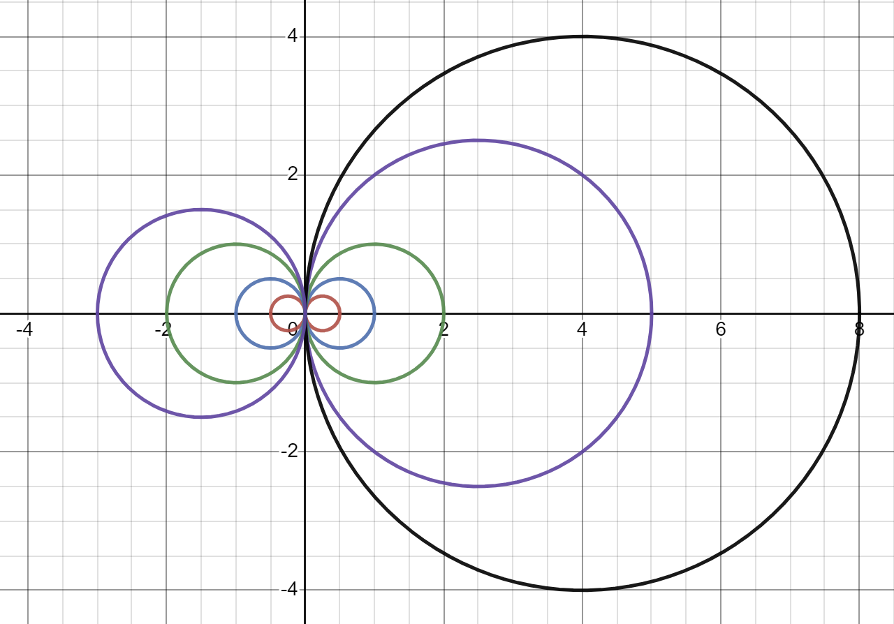
For example, start with the family given by $x^2+y^2=cx$.

Differentiate both sides: $2x+2y\frac{dy}{dx}=c$. Now plug in $c=\frac{1}{x}(x^2+y^2)$ from the original equation, and we get the differential equation:

$$2x+2y\frac{dy}{dx}=\frac{1}{x}(x^2+y^2)\text{which simplifies to}2xy\frac{dy}{dx}+x^2=y^2.$$

Conversely, let us solve this differential equation. Write it as:

$$\frac{dy}{dx}=\frac{y^2-x^2}{2xy}.$$

This is a homogeneous equation, so we can substitute $z=y/x$:

$$\frac{dz}{dx}x+z=\frac{z^2-1}{2z}\text{which implies}\frac{-2z}{z^2+1}dz=\frac{dx}{x}.$$

Integrating both sides, applying $e^{-}$, and substituting $z=y/x$ gives:

$$|x|=\frac{c}{(y/x{)}^2+1}c>0.$$

Now multiply the fraction by $\frac{x^2}{x^2}$ and cross multiply to obtain $|x|(x^2+y^2)=c{x}^2$, which is equivalent to $(x^2+y^2)=c|x|$ assuming $x\ne 0$. Allowing $c\in \mathbb{R}$, we have the original equation.

Link to original

Introduction (part 2)

Something interesting we can do is define the orthogonal family of curves to a given family of curves. The orthogonal family is the family such that each curve is perpendicular to every curve of the original family.

For example, if one family of curves represents electric field lines, its orthogonal family represents equipotential lines. Or, if one family represents the level curves of a function, its orthogonal family represents the lines of steepest ascent.

The orthogonal family can be found from the original family by first computing the differential equation $\frac{dy}{dx}=f(x,y)$. The orthogonal family will be given by the differential equation $\frac{dy}{dx}=-1/f(x,y)$. (The orthogonal slope is the negative reciprocal slope.)

Link to original

Example

Circles and rays

Circles and rays

We verify that the family of rays emanating from the origin is the orthogonal family to the family of circles centered at the origin. The family of circles is given by $x^2+y^2=c$. This corresponds to the differential equation $\frac{dy}{dx}=-\frac{x}{y}$. The orthogonal family is then given by $\frac{dy}{dx}=\frac{y}{x}$. Separating variables: $\frac{dy}{y}=\frac{dx}{x}$ so $\ln |y|=\ln |x|+c$ and thus $y=Cx$ for $C\in \mathbb{R}$. This is the family of rays.

Link to original

Exercises B

Exercise

07

Homogeneous

Solve the following homogeneous equations by substitution of $z=y/x$. You should first write the equation using a single quotient and then divide above and below by $x$.

• (a) $x\sin (y/x)\frac{dy}{dx}=y\sin (y/x)+x$
• (b) $x{y}^{\prime }=2x-6y$

Link to original

Exercise

08

Integrating factors, conversion to exact

Solve the following differential equations by finding an integrating factor $\mu (x)$ or $\mu (y)$.

• (a) $-2xydx+(3x^2-y^2)dy=0$
• (b) $(y\ln y-2xy)dx+(x+y)dy=0$

Link to original

Exercise

09

Bernoulli

Solve the following Bernoulli equation: $x{y}^2{y}^{\prime }+y^3=x\cos x$.

Link to original

Exercise

01

A self-orthogonal family

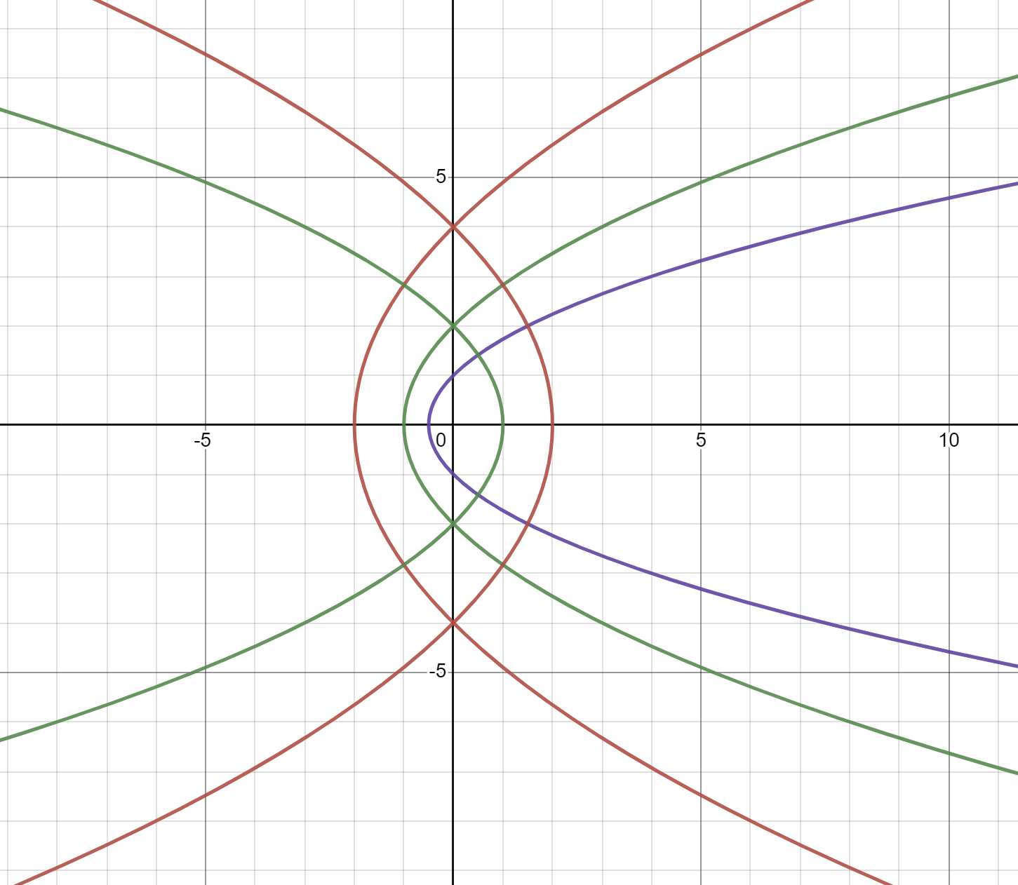
Show that this family of curves is orthogonal to itself: $y^2=4c(x+c)$. (Hint: divide the curves into two families, one with $c>0$ and the other with $c<0$.)
Here’s a picture showing the curves for $c=0.5,1,2$ (opening rightward) and $c=-1,-2$ (opening leftward).

Link to original

Functions and differential equations

Excursus: functions, derivatives, integrals

Excursus - functions, derivatives, integrals

Differentiation and integration are learned as “inverse processes” in calculus, and yet this relationship tends to obscure a fundamental asymmetry between the two concepts. Differentiation has a geometrical meaning that does not rely on the concept of a function, whereas integration cannot be formulated properly without the concept of a function and naturally leads to it.

Given any equation involving $x$ and $y$, we may consider the set of points $(x,y)$ whose coordinates satisfy the equation. For most reasonable equations, this set of points is a curve. Any point on a curve may be associated with a slope, which is the data of the direction of the curve at that point. It is equivalent to the data of the direction of the tangent line passing through the point.

(This association of point to line does not itself have to be a function, since a curve that crosses itself at some point may have two directions associated to the same point, which is disallowed for functions. Incidentally, the example of a curve crossing itself is a good illustration of a problem for the functional perspective which does not obviously have to do with infinity.)

The concept of direction line is a geometrical way of thinking about the derivative, and arguably it is more fundamental than the notion of rate of change. The direction line relates to equations and curves solving the equations. The idea of direction line is also a basic element in the idea of differential equation, since the direction of the direction line is expressed by a relationship between differentials $dy$ and $dx$. One could say that a first-order differential equation is an equation involving points $(x,y)$ as well as the direction lines at those points. A solution to a differential equation is just a curve whose direction line satisfies the differential equation.

The important point here is that the idea of function is somewhat foreign to the concept of derivative and differential equation, at least when the latter are thought of geometrically.

What is a function? A function is a rule, procedure, or method taking inputs to outputs. The essential feature of the idea of function is the difference between input and output, namely the temporal priority of input along with the movement to output according to a specific pattern.

The essence of derivative (direction line) and differential equation (equation involving $dy$ and $dx$) in no way depends on a preferential treatment of $x$ as input and a patterned movement to $y$ as output.

Such is not the case for integration! The essential idea of integration depends on an inequity between the variables, between $x$ which is the independent, prior, input variable, and $y$ which is the dependent, posterior, output variable. The essential idea of integration is to sum up the values of the output with a sum that is weighted by the “quantity of inputs” for which the output has each value. The usual integration in calculus takes the total or sum of outputs $y=f(x)$ weighted by the quantity $dx$ of input near each input value $x$.

A modern consequence of these conceptual differences between derivatives and integrals – between directions and summations – is that modern specialists in algebra and parts of geometry make far greater use of derivatives than they do integrals, whereas modern specialists in analysis, the discipline that studies generalizations of the concept of continuous function, are equally concerned with integrals as with derivatives.

So far our work with differential equations has mostly treated $x$ and $y$ on an equal footing. The main exception is that we have sometimes invoked the chain rule, which depends specifically on the function idea (it is about the composition of functions).

There are many reasons to adopt the functional viewpoint. Most applications of differential equations in mathematical models of physical phenomena rely on this viewpoint. Part of the reason for this is that functions are essential to the concept of rate of change, for which time is a natural independent variable, and functions are used to specify the values of physical quantities at each point in time. The “dynamical system” viewpoint is connected to this one. Numerical techniques are, furthermore, normally framed in functional terms. For these reasons the functional viewpoint is prevalent, ubiquitous, even tacitly assumed, in all applied math contexts.

Another reason to adopt the functional viewpoint is that functions give a type of structure that can encompass both algebraic and non-algebraic relationships. For example, trig functions express geometric relationships, and through the use of functions, algebraic and geometric relationships and quantities can be combined in a single equation. Furthermore, the solutions of differential equations themselves can be incorporated with algebraic and geometric functions in a single equation. For example, $e^x$ or Bessel functions could be included.

In short, when we are interested in mathematical quantity, over and above quality (i.e. abstract structures such as algebraic rules), and we wish to cast everything in terms of quantity, it is useful to adopt the functional viewpoint. We embrace the functional and quantitative viewpoint now and for the remainder of the course. To emphasize this transition, we now write ‘$t$’ by default for our independent variable, and $x$, $y$, $p$, $f(t)$, etc. are all considered to have a functional dependence on $t$.

Link to original

Initial value problems

Initial value problems

A first-order differential equation, from the functional viewpoint, is given by a function $f(t,y)$ that specifies the numerical values of the derivative $y^{\prime }(t)$ in terms of the values of $t$ and $y(t)$. The ODE itself is $y^{\prime }(t)=f(t,y)$. A solution to the ODE is a differentiable function $y(t)$ that satisfies the equation.

Notice: a solution does not mean an equation or anything we might understand or know how to calculate. On the other hand, a solution is now assumed to be a function that returns numbers; this means, for example, that it cannot ever return infinity, since that is not a number.

Since the idea of a differentiable function is easy to define with perfect logical precision, we can ask about a differential equation the logical question of how many solutions exists. If there are infinitely many, we can ask whether there are conditions we can specify that guarantee existence of a unique solution. Taking the functional viewpoint, we typically would like to express such conditions in terms of inputs and outputs of the solution function.

An initial value problem (IVP) is a problem where we specify an initial time $t_0$ and initial values of the function $y_0=y(t_0)$ and possibly a number of its higher derivatives: $y^{\prime }(t_0)$, $y^{\prime \prime }(t_0)$, $\dots$, and ask whether there exists exactly one differentiable function $y(t)$ solving the differential equation and that has these initial values.

The idea of initial value problem also applies in numerical analysis, which is concerned with the development of algorithms that generate approximate solutions for use by computers, because these algorithms typically build approximate solutions by iterating a procedure which extends a partial solution into future time intervals.

Link to original

Functional viewpoint and IVPs: pathological phenomena

Functional viewpoint and IVPs - pathological phenomena

The class of differentiable functions may be easy to define with logical precision, but some innocuous-looking differential equations, even some with reasonable “families of integral curves,” exhibit pathological behaviors from the functional viewpoint.

Vertical asymptote means blowing up: non-existence
It is easy to find a differential equation with IVP starting at $t=0$ whose functional solutions go to infinity in finite time. When this happens, the solution is said to blow up.

Link to original

Example

Solution that blows up

Solution that blows up

Consider the IVP:

$$y^{\prime }(t)=y^2,y(0)=y_0>0.$$

This is a separable differential equation. Assuming $y\ne 0$, we can solve it: $-y^{-1}=t+c$. From the algebraic viewpoint we had been using, the solution to the ODE is the family of curves $(c-t)y=1$, and there is no particular problem with this family.

Now write the solution as a functional solution and solve for the constant using the initial condition $y(0)=y_0$:

$$y(t)=\frac{1}{-t+y_0^{-1}}.$$

Look what happens as time evolves: for $0\le t<y_0^{-1}$, the function $y(t)$ is well-behaved. But as $t\to y_0^{-1}$ we have $y(t)\to +\infty$. In other words, $y(t)$ blows up at $y_0^{-1}$. There is a solution to the IVP (and in fact it is unique when it exists), but the solution cannot be extended beyond the range $t\in (-\infty ,y_0^{-1})$.

This blow-up behavior is not weird algebraically, but functionally it is undesirable, since the solution function does not exist beyond a certain time $t=y_0^{-1}$.

Notice that if the ODE is replaced by $y^{\prime }(t)=-y^2$, then the solution is $y(t)=\frac{1}{t+y_0^{-1}}$, which does not blow up for $t\ge 0$. (Although it does blow up for $t<0$.)

Link to original

Functional viewpoint and IVPs - pathological phenomena (part 2)

Artificial functional solutions: non-uniqueness
Another kind of problem can arise in the functional perspective with a differential equation that poses no difficulties from the algebraic perspective. The problem is that mere “differentiability” is not strong enough to separate out functions that are the same in first derivative, but their higher derivatives may fail to exist.

Link to original

Example

Once-differentiable functions given piecewise, non-uniqueness

Once-differentiable functions given piecewise, non-uniqueness

Consider the IVP:

$$y^{\prime }(t)=2y^{1/2},y(0)=0.$$

This is a separable differential equation: $\frac{1}{2}{y}^{-1/2}dy=dt$ so $y^{1/2}=t+c$. Solving this explicitly: $y=(t+c{)}^2$, and $y=t^2$ is a solution satisfying $y(0)=0$.

But look! Here is a piecewise function, for each $t_0\in \mathbb{R}$, that also solves this IVP:

$$y(t)=\{\begin{array}{ll}(t-t_0{)}^2& t\ge t_0\\ 0& t<t_0.\end{array}$$

Clearly this $y(t)$ is a solution for $t\ne t_0$. Considering $t=t_0$, we have:

$$\begin{array}{rl}\underset{t\to t_0^{+}}{\lim }{y}^{\prime }(t)=\underset{t\to t_0^{+}}{\lim }2(t-t_0)& =0\\ \underset{t\to t_0^{-}}{\lim }{y}^{\prime }(t)=\underset{t\to t_0^{-}}{\lim }0& =0,\end{array}$$

and therefore $y^{\prime }(t_0)$ does exist, namely $y^{\prime }(t_0)=0$, and the ODE is satisfied everywhere.

Notice that $y^{\prime \prime }(t)$ does not exist at $t_0$!

Furthermore, the piecewise solutions are not given by a single equation with parameter, so they do not qualify as a “family of curves” according to our previous usage in the algebraic viewpoint.

Link to original

Functional viewpoint and IVPs - pathological phenomena (part 3)

The family of functional solutions is wild! It can start to increase parabolically at any random time $t_0$ of our choosing. Clearly there is no unique solution to this IVP in the class of differentiable functions. Notice that this non-uniqueness is a local problem, meaning that there is no interval around $t=0$ for which there exists a unique solution. If we desire local uniqueness, then either the differential equation itself is not acceptable, or else our class of functional solutions is too big.

By adopting the functional perspective, we restrict ourselves to objects that are better behaved in one sense – they are well-defined and avoid infinity – but they are worse behaved in another sense: they may exhibit strange behaviors that no algebraic families of curves would, such as non-differentiability, piecewise definitions, random bifurcations, and so on.

Consider the fact that $y^{\prime \prime }(t_0)$ does not exist. Can we fix our problem by restricting functional solutions to the class of functions that are infinitely differentiable, meaning that all their higher derivatives exist and are continuous?

No!!

Link to original

Example

Infinitely differentiable - not enough for uniqueness

Infinitely differentiable: not enough for uniqueness

Consider the IVP: $ydt-t^{2}dy=0,y(0)=0.$

This differential equation is separable, and the solution family is calculated to be $y=C{e}^{-1/t}$ for $C\in \mathbb{R}$. We can also check that $y=0$ is a solution too.

But look! Here is a piecewise function, for each $C\in \mathbb{R}$, that solves the IVP:

$$y(t)=\{\begin{array}{ll}C{e}^{-1/t}& t>0\\ 0& t\le 0.\end{array}$$

At $t=0$ we have $y^{(n)}(t)=0$ for any $n$. For example, from the right $y^{\prime }(t)=\frac{C}{t^2}{e}^{-1/t}$, and this limits to zero as $t\to 0^{+}$. (It is not trivial to prove this, but intuitively the exponential goes to zero much faster than $t^2$ does.)

All these functions are infinitely differentiable, they all satisfy the IVP, and yet they differ from each other for any $t>0$ (for differing $C$ values).

Link to original

Exercise

01

Hopping from a line

Consider the IVP: $y^{\prime }=1+2\sqrt{y-t},y(0)=0$. Show that the (differentiable) functional solutions can extend along the line $y(t)=t$ for arbitrary time in the forward direction, and at some moment deviate from the line following a certain parabola. Can the same happen in the reverse direction?

You are encouraged to understand the differential equation using the Desmos graph at https://www.desmos.com/calculator/sdxp7or83y.

Link to original

Picard-Lindelöf Theorem: local well-posedness

Picard-Lindelöf Theorem - local well-posedness

Our only major theorem in this course is due to Cauchy, Lipschitz, Picard, and Lindelöf. Usually Picard is given most of the credit, but frequently it is called the Picard-Lindelöf theorem.

Picard-Lindelöf Theorem

Suppose the IVP is given by the function $f(t,y)$ and initial value $y_0$:

$$y^{\prime }(t)=f(t,y),y(t_0)=y_0,$$

and suppose that $f(t,y)$ has the following properties: there is some rectangle $D=(a,b)\times (c,d)$ containing $(t_0,y_0)$, and numbers $B,C>0$ such that:

$$|f(t,y)|\le B\text{and}\left|\frac{f(t,y_2)-f(t,y_1)}{y_2-y_1}\right|\le C\text{ on }D.$$

Then there exists a unique local solution to this IVP.

Here the precise meaning of local solution is that there is some interval $t_0-\epsilon <t<t_0+\epsilon$ for which a solution exists. The local solution is unique in the sense that any other local solution must agree with this solution on some interval (possibly smaller).

Variants of Picard-Lindelöf

• If we know that $f(t,y)$ and $\frac{\partial f}{\partial y}$ are both continuous on some rectangle $D$ containing $(t_0,y_0)$, then there exists a unique local solution to this IVP.
• If we know that $f(t,y)$ and $\frac{\partial f}{\partial y}$ are both bounded on some rectangle $D$ containing $(t_0,y_0)$, then there exists a unique local solution to this IVP.

These statements follow from the first version using the Mean Value Theorem and some topological arguments that we omit.

Picard-Lindelöf does not prevent blowups!

The Picard-Lindelöf theorem only provides local solutions, meaning some interval which is potentially microscopic on which the solution exists. These intervals could become arbitrarily small as you approach a blowup point. They do not guarantee solutions that extend beyond a blowup point!

On the other hand, the Picard-Lindelöf theorem does prevent the artificial piecewise solutions we have seen which exhibit non-uniqueness. How? Those IVPs do not meet the conditions of Picard-Lindelöf! In other words, instead of trimming away bad functional solutions, the theorem excludes those IVPs because the differential equations themselves are excluded.

Link to original

Example

Picard-Lindelöf frequently not applicable

Picard-Lindelöf frequently not applicable

The IVP $y^{\prime }(t)=2y^{1/2},y(0)=0$ does not satisfy Picard-Lindelöf. We have $\frac{\partial f}{\partial y}=\frac{1}{\sqrt{y}}$, and this is neither continuous nor bounded on any interval containing $(0,0)$. So the “Variants” of Picard-Lindelöf do not apply. Furthermore, the difference quotient can be made arbitrarily large by letting it approximate this partial near $(0,0)$, so the original Picard-Lindelöf does not apply either.

Link to original

Picard-Lindelöf Theorem - local well-posedness (part 2)

Conclusion: the Picard-Lindelöf theorem restricts us to IVPs with $y^{\prime }(t)=f(t,y)$ such that $f(t,y)$ is nicely behaved near the initial data $(t_0,y_0)$. Critically, this means the partial $f_y$ should be nicely behaved there too.

Link to original

Picard iteration

Picard iteration

The Picard-Lindelöf theorem is proven by developing a sequence of functional solution candidates, and showing that they converge to a real solution, and furthermore that any other solution must converge (locally) to the same one. Functions in this sequence are called Picard iterates because the sequence is produced by an iterative process.

The Picard iteration procedure can be computed by hand for some interesting cases, and it is worthwhile to do so. To that end, let us set up the process in general.

From the functional viewpoint, an IVP is given by $y^{\prime }(t)=f(t,y)$ and $y(t_0)=y_0$. It is convenient to assume that $(t_0,y_0)=(0,0)$. (If this is not the case, you can change variables and write a new IVP in the new variables that does satisfy this property.) So the IVP is now $y^{\prime }(t)=f(t,y)$ and $y(0)=0$.

Suppose $y(t)$ is a solution to the IVP. Integrate both sides:

$$y(t)={\int }_0^{t}f(s,y(s))ds.$$

Now suppose $y(t)$ is a function that satisfies the above integral equation, and differentiate both sides. By the Fundamental Theorem of Calculus, we obtain $y^{\prime }(t)=f(t,y(t))$ and $y(0)=0$. Therefore, the integral equation above is equivalent to the original IVP.

Notice that this translation to an integral equation relies critically on the functional viewpoint!

Ponder the format of this integral equation. It says that if we apply the operation ${\int }_0^{-}f(s,-(s))ds$ to the function $y(t)$, then we get back the same function $y(t)$. In other words, $y(t)$ is preserved or fixed by this operation.

The general strategy to show that there is a unique solution is to show that there can be only one fixed point of this operation acting upon the class of differentiable functions. (The reason is that the operation is “shrinking,” in a sense that we cannot explain fully here, but the rough idea is that it pulls candidate functions closer and closer together.)

The strategy to show that a solution exists is to start with any candidate function and apply the operation repeatedly, and the candidate will be pulled closer and closer to the fixed point of the operation, namely to the solution of the IVP. To notate this, let $y_0(t)$ be any initial candidate solution. Then we define:

$$\begin{array}{rl}{y}_1& ={\int }_0^{t}f(s,y_0)ds\\ y_2& ={\int }_0^{t}f(s,y_1)ds\\ y_3& ={\int }_0^{t}f(s,y_2)ds\\ & ⋮\\ y_n& ={\int }_0^{t}f(s,y_{n-1})ds.\end{array}$$

We expect that $y_n(t)\to y(t)$ as $n\to \infty$, for $y(t)$ a solution to the IVP.

Link to original

Example

Picard iteration can yield an exact solution

Picard iteration can yield an exact solution

Consider the IVP $y^{\prime }=2y,y(0)=1$. Change variables to $z=y-1$ and get the IVP $z^{\prime }=2(z+1)$ and $z(0)=0$. Set $z_0(t)=0$ and iterate:

$$\begin{array}{rl}{z}_1& ={\int }_0^{t}f(s,0)ds={\int }_0^{t}2ds=2t\\ z_2& ={\int }_0^{t}f(s,z_1)ds={\int }_0^{t}2(2s+1)ds=2t^2+2t\\ z_3& ={\int }_0^{t}f(s,z_2)ds={\int }_0^{t}2(2s^2+2s+1)ds=\frac{4}{3}{t}^3+2t^2+2t\\ & ⋮\\ z_n& ={\int }_0^{t}f(s,z_{n-1})ds={\int }_0^{t}2(z_{n-1}+1)ds.\end{array}$$

So we conclude that $z(t)$ is given by the power series

$$z(t)=2t+2t^2+\frac{4}{3}{t}^3+\frac{2}{3}{t}^4+\dots$$

and the coefficients are defined recursively by $a_1=2$, $a_n=\frac{2}{n}{a}_{n-1}$. This recursion relation is solved by the general term $a_n=\frac{2^n}{n!}$, so we have:

$$\begin{array}{rl}z(t)& =0+\frac{(2t)}{1!}+\frac{(2t{)}^2}{2!}+\frac{(2t{)}^3}{3!}+\dots \\ & =e^{2t}-1.\end{array}$$

Link to original

Picard iteration (part 2)

We found an exact solution by:

• computing Picard iterates,
• observing a growing power series,
• identifying a recursion relation,
• solving the recursion relation for the general coefficient,
• recognizing a known power series.

Sometimes the last step or two cannot be accomplished, but in principle the first three steps can always be done.

Link to original