Chapter 16 - Partial Derivatives and Optimization

Partial Derivatives

Introduction

Suppose we are given a function $f:{\mathbb{R}}^2\to \mathbb{R}$, written in terms of components by $f(x,y)\in \mathbb{R}$ for each $(x,y)\in {\mathbb{R}}^2$. Now let the second coordinate remain some arbitrary fixed value $y=b$. This determines a function $f(x,b)$ of one variable, $x$, for each possible chosen $b$.

We can take the derivative of $f(x,y_0)$ in $x$ just as any other function of $x$:

$$\frac{d}{dx}f(x,b)=\underset{h\to 0}{\lim }\frac{f(x+h,b)-f(x,b)}{h}.$$

The resulting function of $x$ may be considered for various possible values of $b$, i.e. the variation may be restored. This function of both $x$ and $y$ is called the partial derivative of $f$ with respect to $x$. As with ordinary derivatives, a variety of notations is used:

$$f_x(x,y)=\frac{\partial }{\partial x}f(x,y)=\frac{\partial f}{\partial x}(x,y)=\underset{h\to 0}{\lim }\frac{f(x+h,y)-f(x,y)}{h}.$$

The new symbol ‘ $\partial$ ’ is called “partial” and should be written differently from ‘ $d$ ’. This symbol indicates the function’s dependence on additional variables.

Functions of several variables may have partial derivatives in each of their variables. Thus, for $f$ above we also have $f_y$ or $\frac{\partial f}{\partial y}$.

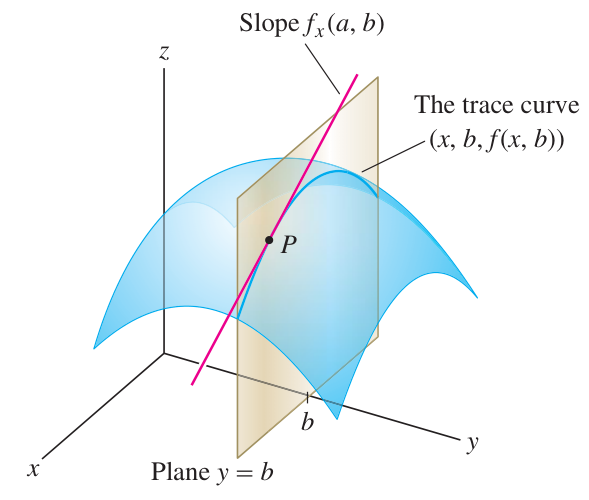
By interpreting the function $f(x,b)$ as the “trace” of the function $f(x,y)$ at a fixed value $y=b$, one sees that the partial derivative gives the slope of the curve formed as the cross-section of the plane $y=b$ with the graph of $f$, namely the surface $z=f(x,y)$:

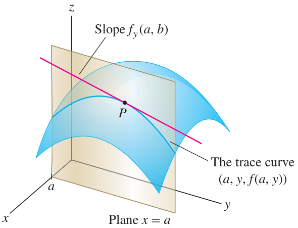
Similarly for the partial $f_y$ and the trace $x=a$:

One can iterate partial derivatives and consider higher partials in the obvious manner. The notation $f_{xy}$ indicates the “mixed partial” taken in $x$ first:

$$f_{xy}=\frac{\partial }{\partial y}\left(\frac{\partial f}{\partial x}\right)=\frac{{\partial }^{2}f}{\partial y\partial x}.$$

In principle, the double partials $f_{xy}$ and $f_{yx}$ could be different, but for nice functions they do agree by Clairaut’s Theorem:

Clairaut’s Theorem

Provided $f_{xy}$ and $f_{yx}$ exist and are continuous on a region $\mathcal{R}$, then $f_{xy}=f_{yx}$ on that region.

(Caveat: in the theorem, $\mathcal{R}$ should be ‘open’ topologically: it should have the same dimension as the background and not include its boundary.)

Link to original

Example

Partial derivatives of a monomial

Partial derivatives of a monomial

Problem: Compute the partial derivatives of first and second order of the function $f(x,y)=x^3{y}^5$.
Solution: We have $f_x=3x^2{y}^5$, $\frac{\partial f}{\partial y}=5x^3{y}^4$, $f_{xy}=f_{yx}=15x^2{y}^4$, $\frac{{\partial }^{2}f}{\partial x^2}=6x{y}^5$, $f_{yy}=20x^3{y}^3$.

Link to original

Exercise

01

Partial derivatives of a composite

Let $f(x,y)=\sin (\frac{x}{1+y})$. Compute $\frac{\partial f}{\partial x}$ and $\frac{\partial f}{\partial y}$.

Link to original

Exercise

02

Evaluate partial with four variables

Let

$$f(x,y,z,w)=\frac{e^{xz+y}}{z^2+w}.$$

Calculate $f_z(0,0,1,1)$.

Link to original

Exercise

03

Higher order partials

Let $f(x,y,z)=x^3+y^2{e}^x$.

• (a) Calculate the second-order partial derivatives of $f$.
• (b) Calculate $f_{xyy}$.

Link to original

Exercise

04

Clairaut: choose the order wisely!

Let $f(x,y,z,w)=x^3{w}^2{z}^2+\sin (\frac{xy}{z^2})$. Compute $f_{zzwx}$ in your head. (Explain it on paper!)

Link to original

Introduction (part 2)

Continuity and differentiability: more complex in 3d!

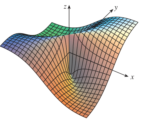
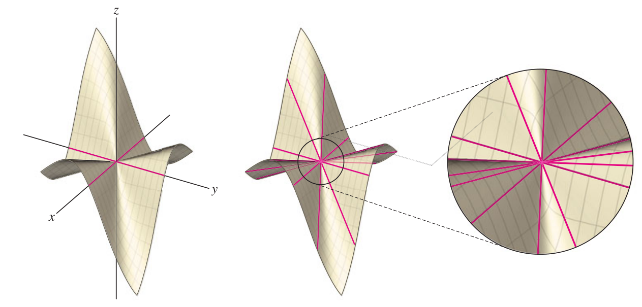
The concepts of continuity and differentiability are more complicated in 3d due to potential incompatibilities of directionality that are a function of the $x$ and $y$ relationship.
$z=f(x,y)=\frac{xy}{x^2+y^2}$

$z=f(x,y)=\frac{2xy(x+y)}{x^2+y^2}$

Link to original

Linear approximation

Introduction

There is a relation between the concepts of linear approximation, partial derivative, tangent plane, and differentiability. This relation is contained in a function defined in terms of $f(x,y)$:

Linear approximation function

$$L(x,y)=f(a,b)+f_x(a,b)\cdot (x-a)+f_y(a,b)\cdot (y-b).$$

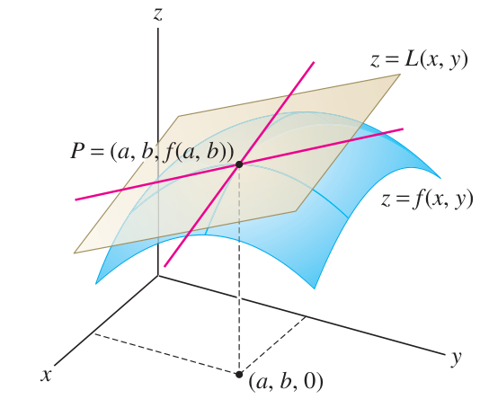
The linear approximation function includes both partial derivatives $f_x$ and $f_y$. The set of points satisfying $z=L(x,y)$ defined by the above equation, namely the graph of $L(x,y)$, is the tangent plane. Lastly, the function $f(x,y)$ is said to be differentiable when:

$$f(x,y)=L(x,y)+(x-a)\cdot {\epsilon }_1+(y-b)\cdot {\epsilon }_2,$$

with two functions ${\epsilon }_1$ and ${\epsilon }_2$ satisfying ${\epsilon }_1,{\epsilon }_2\to 0$ as $(x,y)\to (a,b)$.

If $f(x,y)$ is not differentiable, then the linear approximation may be a bad approximation.

Linear approximation in 2d

Remember that for a function $f(x)$ of a single variable, we have the linear approximation:

$$L(x)=f(a)+f^{\prime }(a)\cdot (x-a).$$

The tangent line to $f$ at $x=a$ is given by $y=L(x)$, and $f$ is considered differentiable when $f(x)=L(x)+(x-a)\cdot \epsilon$ such that $\epsilon \to 0$ as $x\to a$:

$$\left(\frac{f(x)-f(a)}{x-a}-f^{\prime }(a)\right)=\epsilon \to 0\text{ as }x\to a\text{iff }{f}^{\prime }(x)\text{ exists at }a.$$

Tangent plane via tangent lines

How do we know that the graph of $L(x,y)$ gives the tangent plane?

The tangent vector to the trace $z=f(x,b)$ at $x=a$ is given by ${\frac{d}{dx}(x,b,f(t,b))|}_a=(1,0,f_x(a,b))$. So the tangent line is given by:

$${\mathbf{q}}_{(a,b)}(t)=(a,b,f(a,b))+t(1,0,f_x(a,b))=(a+t,b,f(a,b)+t{f}_x(a,b)).$$

These points satisfy $z=L(x,y)$. The graph $z=L(x,y)$ must be the tangent plane because it is the unique plane such that the tangent lines of the trace curves $f(x,b)$ and $f(a,y)$ lie in this plane.

Taylor series and linear approximation

Linear approximation gives the first two terms of the Taylor series of a function, and the remainder term, captured in $\epsilon$, must limit to zero when the function is differentiable:

$$\begin{array}{rl}f(x)& =f(a)+f^{\prime }(a)(x-a)+\frac{1}{2!}{f}^{\prime \prime }(a)(x-a{)}^2+\dots \\ & =f(a)+f^{\prime }(a)(x-a)+\epsilon \cdot (x-a).\end{array}$$

If $f$ agrees with its Taylor series, then:

$$\epsilon (x)=\frac{1}{2!}{f}^{\prime \prime }(a)(x-a)+\frac{1}{3!}{f}^{(3)}(a)(x-a{)}^2+\frac{1}{4!}{f}^{(4)}(x-a{)}^3+\dots$$

Link to original

Differentials

Differentials

Some authors use the mnemonic notation of finite differentials for applications of linear approximation. These are written as $dx$, $dy$, $dz$, $df$, etc., even though they are not infinitesimals. Their usage is according to the following kind of rules:

$$df=\frac{\partial f}{\partial x}dx+\frac{\partial f}{\partial y}dy.$$ Link to original

Example

Tangent plane to paraboloid

Tangent plane to paraboloid

Problem: Find the equation of the plane tangent to the paraboloid $z=2x^2+y^2$ at $(x,y,z)=(1,1,3)$.
Solution: Set $f(x,y)=2x^2+y^2$. Compute $f_x=4x$, $f_y=2y$. So $f_x(1,1)=4$, $f_y(1,1)=2$, and the linear approximation is given by:

$$L(x,y)=3+4(x-1)+2(y-1).$$

The tangent plane is found by setting $z=L(x,y)$.

Link to original

Exercise

01

Tangent plane to a graph

Let $f(x,y)=x{y}^3+x^2$. Find the tangent plane to the graph of $f(x,y)$ at the point $(x,y)=(2,-2)$.

Link to original

Exercise

02

Linear approximation

Use a linear approximation to estimate the value of $(3.99{)}^3(1.01{)}^4(1.98{)}^{-1}$.

• (a) Write this using a function $L(x,y,z)$.
• (b) Write this using the notation of differentials.

What is the percentage error of your estimate from the true value?

Link to original

Differentiability

Differentiability

In 2d, a function $f(x)$ is differentiable precisely where its derivative $f^{\prime }(x)$ exists. The situation is not so simple in 3d: a function like $f(x,y)=\frac{2xy(x+y)}{x^2+y^2}$ has both partial derivatives at $(x,y)=(0,0)$, but it is not differentiable there! On the other hand, one theorem does help:

Theorem

If a function $f(x,y)$ is given and both partials $f_x$ and $f_y$ exist and are continuous at a point $(a,b)$, then $f$ is differentiable at $(a,b)$.

Link to original

Exercise

03

When partials aren’t continuous

Compute the partial derivatives of $f(x,y)=\frac{2xy(x+y)}{x^2+y^2}$ and explain carefully why this non-differentiable function does not violate the theorem.

Link to original

Exercise

04

Differentiability of the radius function

Let $r(x,y)=\sqrt{x^2+y^2}$. Is $r(x,y)$ differentiable? Where?

Link to original

Differentiability (part 2)

Differentiable, but partials aren’t continuous: $r^2\sin (\frac{1}{r})$

The function $f(r,\theta )=r^2\sin (\frac{1}{r})$ is differentiable at $(0,0)$ since it is approximated by its tangent plane at $(0,0)$. The partials are not continuous there! You may check this by computing $f_x$ and $f_y$. You can also compute $f_r=2r\sin (1/r)-\cos (1/r)$, which is not continuous at $r=0$.

Link to original

Chain Rule

Chain rule over a curve

Chain rule over a curve

Suppose $f(x,y)$ is a real-valued function on the plane, and $\mathbf{r}(t)=(x(t),y(t))$ is a parametric curve. There is a recipe to compute the derivative of the composite function $(f\circ \mathbf{r})(t)=f(x(t),y(t))$:

$$\frac{d}{dt}f(x,y)=\frac{\partial f}{\partial x}\frac{dx}{dt}+\frac{\partial f}{\partial y}\frac{dy}{dt}.$$ Link to original

Example

Particle moving through temperature gradient

Particle moving through temperature gradient

Problem: A particle traverses a parametric curve in the plane given by $\mathbf{r}(t)=(\cos (t),e^t)$. The ambient temperature is a function of distance from the $y$-axis: $T(x,y)=\frac{1}{x^2+3}$. How fast is the temperature changing at $t=4$?
Solution: We compute $\frac{\partial T}{\partial x}=\frac{-2x}{(x^2+3{)}^2}$ and $\frac{\partial T}{\partial y}=0$, while $x^{\prime }(t)=-\sin (t)$. Then:

$$\frac{df}{dt}=\frac{2\cos (t)\sin (t)}{({\cos }^2(t)+3{)}^2},{\frac{df}{dt}|}_{t=4}=\frac{2\cos (4)\sin (4)}{({\cos }^2(4)+3{)}^2}\approx \mathrm{0.084.}$$

Link to original

Chain rule over a curve (part 2)

Derivation of chain rule over a curve

Let’s suppose that some small change $\Delta t$ produces a change $\Delta x$ and $\Delta y$ via the parametrization $\mathbf{r}(t)$. By differentiability of $f$, we have:

$$\Delta f=\frac{\partial f}{\partial x}\Delta x+\frac{\partial f}{\partial y}\Delta y+\Delta x\cdot {\epsilon }_1+\Delta y\cdot {\epsilon }_2.$$

Divide both sides by $\Delta t$, and take the limit as $\Delta t\to 0$. Notice that ${\epsilon }_1\to 0$ and ${\epsilon }_2\to 0$ because $\Delta t\to 0$ implies $\Delta x,\Delta y\to 0$. It follows that we have:

$$\frac{\Delta f}{\Delta t}\to \frac{df}{dt}=\frac{\partial f}{\partial x}\frac{dx}{dt}+\frac{\partial f}{\partial y}\frac{dy}{dt}+\frac{dx}{dt}\cdot 0+\frac{dy}{dt}\cdot 0.$$

So the sum of products in this chain rule comes from the linear approximation formula, which in turn comes from the tangency of the trace curves.

Link to original

Chain rule over several parameters

Chain rule over several parameters

The chain rule over a curve can be used to derive a more general chain rule for the case when the input variables are functions of several parameters. The formulas can be remembered as “sum of all products” (considering all products that make sense).

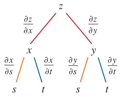
Suppose $f(x,y)$ is a function, and suppose $x(s,t)$ and $y(s,t)$ are both functions of $s$ and $t$. We can “consider” $f$ itself to be a function of $s$ and $t$ via the composition. Then:

$$\begin{array}{rl}\frac{\partial f}{\partial s}& =\frac{\partial f}{\partial x}\frac{\partial x}{\partial s}+\frac{\partial f}{\partial y}\frac{\partial y}{\partial s},\\ \frac{\partial f}{\partial t}& =\frac{\partial f}{\partial x}\frac{\partial x}{\partial t}+\frac{\partial f}{\partial y}\frac{\partial y}{\partial t}.\end{array}$$

These formulas may be derived immediately from the formula for the chain rule over a curve by considering the trace curves: let $t=b$ remain fixed for the first equation, and let $s=a$ remain fixed for the second equation.

Link to original

Exercise

01

Chain rule, several parameters

Let $f(x,y,z)=xy+z$ and $x=s^2$, $y=st$, and $z=s{t}^2$.

• (a) Generalize the chain rule above to the case of 3 variables and compute the partials $\frac{\partial f}{\partial s}$ and $\frac{\partial f}{\partial t}$.
• (b) Write out $f$ in terms of $s$ and $t$ and compute the same partials directly.

Link to original

Example

Polar partials and chain rule

Polar partials and chain rule

Problem: Suppose $f(x,y)$ is a real-valued function of points in the plane. Let $r$ and $\theta$ be the standard polar coordinates on the plane.

• (a) Write $\frac{\partial f}{\partial \theta }$ in terms of $\frac{\partial f}{\partial x}$ and $\frac{\partial f}{\partial y}$ and $x$ and $y$.
• (b) Suppose $f=x^2{y}^3$. Find $f_{\theta }$ at $(x,y)=(1,1)$.

Solution: (a) First compute $\frac{\partial x}{\partial \theta }=-r\sin (\theta )$ and $\frac{\partial y}{\partial \theta }=r\cos (\theta )$. Then:

$$\begin{array}{rl}\frac{\partial f}{\partial \theta }& =\frac{\partial f}{\partial x}\frac{\partial x}{\partial \theta }+\frac{\partial f}{\partial y}\frac{\partial y}{\partial \theta }\\ & =-r\sin (\theta )\frac{\partial f}{\partial x}+r\cos (\theta )\frac{\partial f}{\partial y}\\ & =-y\frac{\partial f}{\partial x}+x\frac{\partial f}{\partial y}.\end{array}$$

(b) Compute $f_x=2x{y}^3$, $f_y=3x^2{y}^2$. So $f_{\theta }=-2x{y}^4+3x^3{y}^2$ and $f_{\theta }(1,1)=-2+3=1$.

Link to original

Exercise

02

Polar partials

Write $\frac{\partial f}{\partial r}$ in terms of $\frac{\partial f}{\partial x}$ and $\frac{\partial f}{\partial y}$ and $x$ and $y$.

Link to original

Chain rule over several parameters (part 2)

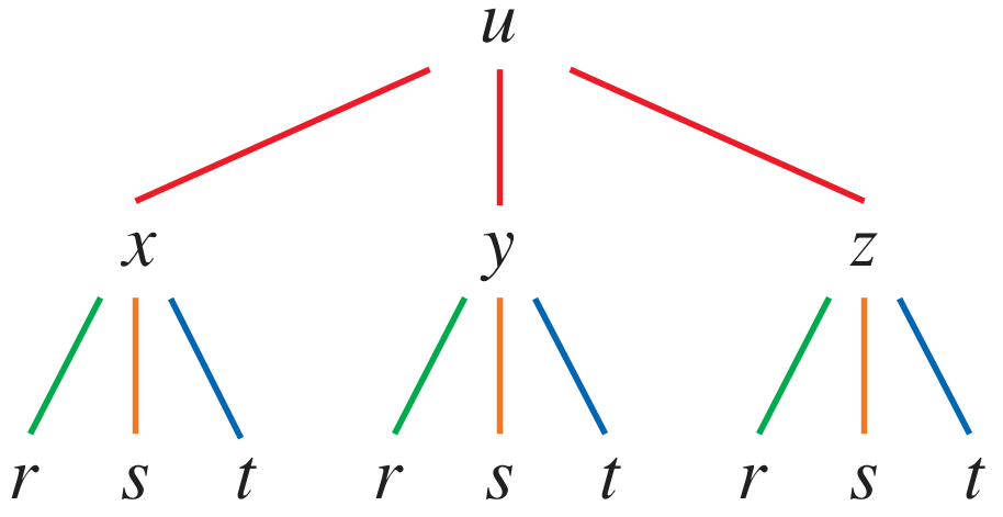
It is easy to generalize the chain rule to an arbitrary number of variables and parameters. Formally, the rule is:

$$\frac{\partial f}{\partial t_i}=\frac{\partial f}{\partial x_1}\frac{\partial x_1}{t_i}+\frac{\partial f}{\partial x_2}\frac{\partial x_2}{t_i}+\cdots +\frac{\partial f}{\partial x_n}\frac{\partial x_n}{t_i},$$

where $f(x_1,x_2,\dots ,x_n)$ is a function of many variables, and each $x_{\ell }(t_1,t_2,\dots ,t_k)$ is a function of many parameters.

To remember the formula, it sometimes helps to draw a tree. The summation has one term for each path from the output variable $z=f(x,y)$ down to the relevant input variable:

Link to original

Exercise

03

Chain rule: 3 variables, 3 parameters

Find $\frac{\partial u}{\partial s}$ at the point $(r,s,t)=(2,1,0)$ given that:

$$u=x^{4}y+y^2{z}^3,x=rs{e}^t,y=r{s}^2{e}^{-t},z=r^{2}s\sin (t).$$

Link to original

Directional derivative

Introduction

The partial derivative $\frac{\partial f}{\partial x}$ gives the rate of change of $z=f(x,y)$ with respect to the variable $x$.

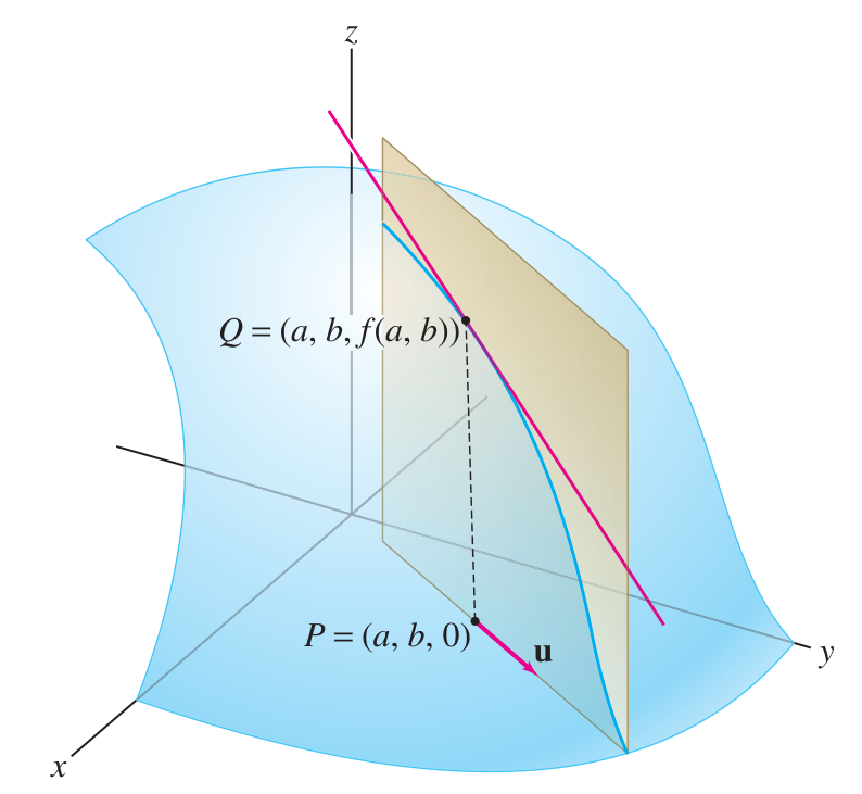
Think of $x$ as a coordinate that moves the input to the function along a line $(x,b)$. The partial $f_x$ gives the rate of change of $f$ with respect to this coordinate.

We can move along other lines, at other speeds. Let $\mathbf{v}$ be any vector in the $xy$-plane. Consider the line $L_{\mathbf{v}}(t)=(a,b)+t\mathbf{v}$ that starts at $(a,b)$ and moves along $\mathbf{v}$ using the parameter $t$. We can take the derivative of $f$ with respect to $t$, and the result is called the derivative of $f$ with respect to the vector $\mathbf{v}$. Here is the defining formula:

$$D_{\mathbf{v}}f(a,b)=\frac{d}{dt}f(\mathbf{L}(t))=\underset{t\to 0}{\lim }\frac{f(a+th,b+tk)-f(a,b)}{t},$$

where we write $\mathbf{v}=(h,k)$ for the components of $\mathbf{v}$.

Observe that the directional derivatives $D_{{\mathbf{e}}_{\mathbf{i}}}(f)$ and $D_{{\mathbf{e}}_{\mathbf{j}}}(f)$ with respect to the unit vectors are identical with the partial derivatives $f_x$ and $f_y$. (Plug in ${\mathbf{e}}_{\mathbf{i}}=(1,0)$ into the limit formula above, for example.)

Link to original

Exercise

01

Linearities of directional derivative

• (a) Show that $D_{\mathbf{v}}(\lambda f+g)=\lambda \cdot D_{\mathbf{v}}f+D_{\mathbf{v}}g$.
• (b) Show that $D_{\lambda \cdot \mathbf{v}}f=\lambda \cdot D_{\mathbf{v}}f$.

Link to original

Introduction (part 2)

Lengthening the direction vector

Notice that the derivative of $f$ with respect to a vector $2\mathbf{v}$ is twice the derivative of $f$ with respect to $\mathbf{v}$. This is because the line $L_{2v}$ is the same line as $L_{\mathbf{v}}$ but traversed twice as quickly.

Calculating directional derivatives
We can use the two partial derivatives $f_x$ and $f_y$ to calculate $D_{\mathbf{v}}f$ for vectors $\mathbf{v}$ other than coordinate basis vectors ${\mathbf{e}}_{\mathbf{i}}$ and ${\mathbf{e}}_{\mathbf{j}}$. Recall $\mathbf{v}=(h,k)$. Use the chain rule instead of the limit definition to compute:

$$\begin{array}{rl}{D}_{\mathbf{v}}f(a,b)& ={\frac{d}{dt}f(\mathbf{L}(t))|}_{t=0}\\ & =f_x(a,b)\cdot x^{\prime }(0)+f_y(a,b)\cdot y^{\prime }(0)\\ & =f_x(a,b)\cdot h+f_y(a,b)\cdot k.\end{array}$$ Link to original

Example

Derivative with respect to a vector

Derivative with respect to a vector

Problem: Find the derivative of $f(x,y)=x{e}^y$ at the point $(2,-1)$ with respect to the vector $\mathbf{v}=(2,3)$.
Solution: The partials at $(2,-1)$ are given by $f_x=e^y=e^{-1}$ and $f_y=x{e}^y=2e^{-1}$. So we calculate $D_{\mathbf{v}}(f)(2,-1)=e^{-1}\cdot 2+2e^{-1}\cdot 3\approx 2.94$.

Link to original

Introduction (part 3)

Unit vectors?

Many authors treat directional derivatives as if they only make sense with respect to unit vectors: $D_{\mathbf{u}}(f)$. If you are interested in the analogue of partial derivative for other directions, you will want to take unit vectors. It may be reasonable to reserve the word ‘directional’ for this case, but it is certainly beneficial to allow the notation $D_{\mathbf{v}}$ to extend to vectors $\mathbf{v}$ that do not have unit length.

Link to original

Example

Directional derivative

Directional derivative

Problem: Find the ‘directional’ derivative of $f(x,y)=x{e}^y$ at the point $(2,-1)$ in the direction of the vector $\mathbf{v}=(2,3)$.
Solution: The key phrase “in the direction of” suggests that we need the unit vector in the direction of $\mathbf{v}$. The norm of $\mathbf{v}$ is $\sqrt{13}$, so we want $D_{\frac{1}{\sqrt{13}}\mathbf{v}}(f)$. By the linearity rule with $\lambda =\frac{1}{\sqrt{13}}$, we can just multiply the previous result by $\frac{1}{\sqrt{13}}$, obtaining $0.82$.

Link to original

Exercise

02

Directional derivative

Suppose $f(x,y,z)=10+y{z}^2+x^{2}z-x{y}^2$. Find the rate of change of $f$ at the point $(1,2,1)$ in the direction of the vector $(0,1,1)$.

Link to original

Optimization

Review of 1D theory

Review of 1D theory

A regular point of a function $f$ is a point $c$ where $f^{\prime }(c)=m\ne 0$. A critical point is a point $c\in \mathbb{R}$ where $f^{\prime }(c)$ is either zero or undefined. In calculus, the theory of optimization (finding extremal values) is largely a theory of critical points.

Given a function $f(x)$ of a single variable, its extrema occur either on boundary points of the region, or at critical points of $f$ in the interior of the region. For a closed interval $[a,b]$, the boundary points are $a$ and $b$, while the interior is the open interval $(a,b)$. Every interior point is either regular or critical. To find extrema, therefore, it suffices to check boundary points, interior points of non-differentiability, and interior points where the derivative is zero.

All of this reasoning may be derived from the linear approximation:

Linear approximation: $f^{\prime }(c)\ne 0⟹\text{local increase/decrease possible}$

If $f^{\prime }(x)$ exists at $c$, we can write $f$ near $c$ as:

$$f(x)=b+m\Delta x+\Delta x\epsilon (\Delta x).$$

Here $f(c)=b$, $f^{\prime }(c)=m$, and $\Delta x=x-c$. Now rewrite this as $f(x)=b+(m+\epsilon )\Delta x$. If $m>0$, then for $\Delta x$ small enough, $m+\epsilon >0$ because $\epsilon \to 0$ as $\Delta x\to 0$. This means there are points $a$ close to $c$ for which $f(a)>f(c)$ (with $a>c$), and points for which $f(a)<f(c)$ (with $a<c$). Conversely, if $m<0$, there are points $a$ near $c$ for which $f(a)<f(c)$ and for which $f(a)>f(c)$.

It follows that if $c$ is a regular point, meaning $f^{\prime }(c)=m\ne 0$, then $c$ is certainly neither a local maximum nor minimum.

The critical points can be evaluated using the first and second derivative tests. For example, if the sign of $f^{\prime }$ crosses zero at $c$ from above, or if $f^{\prime \prime }(c)<0$, the point is a local maximum.

Link to original

2D theory

2D theory

The 1D theory may be applied directly to the trace curves of a function $f(x,y)$, i.e. the curves given by $z=f(x,b)$ or $z=f(a,y)$. The result is that if $f_x(a,b)=m_x\ne 0$, or if $f_y(a,b)=m_y\ne 0$, then $(a,b)$ is neither a local maximum nor minimum, but rather it would be possible to increase or decrease $f$ by moving along the respective trace curve.

A critical point of $f(x,y)$ is a point $(a,b)$ such that either $f_x(a,b)=f_y(a,b)=0$, or at least one of $f_x,f_y$ doesn’t exist. All extreme values of $f(x,y)$ in the interior of a region must occur, therefore, at critical points.

(Note: the situation where, say, $f_y$ fails to exist while $f_x=m_x\ne 0$, counts as a critical point in these notes, but some other authors would not count it. Such points cannot be local extrema by the trace-curve reasoning applied to $x$.)

The definition of critical points can be encapsulated in a single statement about the gradient:

Info

The point $p$ is a critical point of $f$ if and only if: $\nabla f(p)=\vec{0}$ or $\nabla f(p)$ is undefined.

Global extrema are either local extrema (critical points in the interior), or they lie on the boundary. To check the boundary, one must find a parametrization of the boundary as a curve $\mathbf{r}(t)$, and then optimize the scalar function $f(\mathbf{r}(t))$ of the single variable $t$ using the 1D theory. The extrema on the boundary should then be compared with the local extrema in the interior.

As in the 1D theory, critical points of $f(x,y)$ can be either maxima or minima or neither, and there is a tool involving second-order partials that allows us to classify critical points in many cases. It is called the discriminant. Suppose that $f_{xx},f_{yy},f_{xy}$ exist and are continuous near $(a,b)$, a critical point of $f(x,y)$. Define the discriminant $D(x,y)$ by the formula:

$$D(x,y)=f_{xx}(x,y)f_{yy}(x,y)-f_{xy}(x,y{)}^2.$$

This formula is easy to remember as the determinant of the matrix of second-order partials:

$$D=\left|\begin{array}{cc}{f}_{xx}& f_{xy}\\ f_{yx}& f_{yy}\end{array}\right|.$$

Discriminant test

Let $(a,b)$ be a critical point near which the second-order partials are continuous.

• If $D(a,b)=0$ the test is inconclusive
• If $D(a,b)<0$ then $(a,b)$ is a saddle point
• If $D(a,b)>0$ then $(a,b)$ is a max/min:
  • If $f_{xx}>0$ or $f_{yy}>0$ then $(a,b)$ is a min
  • If $f_{xx}<0$ or $f_{yy}<0$ then $(a,b)$ is a max

Link to original

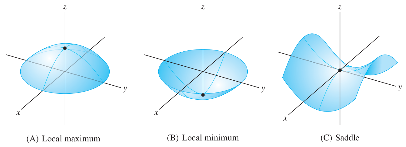
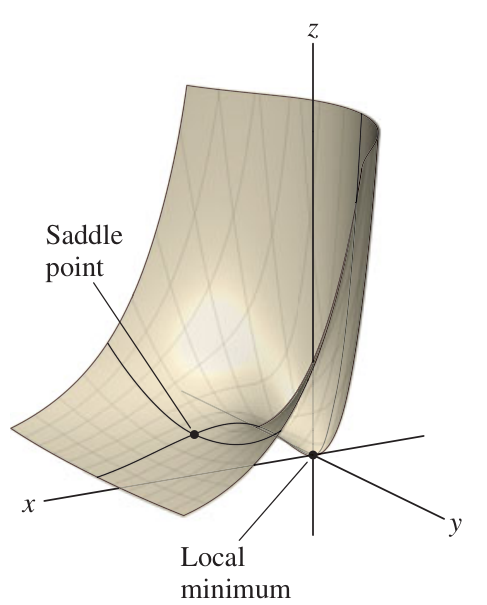
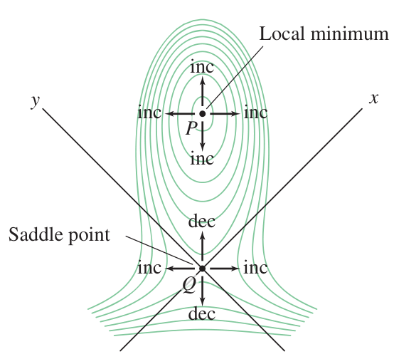
Exercise

01

Classify critical points on topographical contour map

Link to original

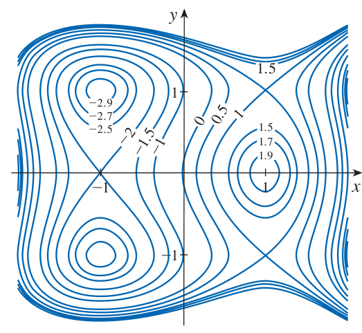
Example

Minimum vs. saddle

Minimum vs. saddle

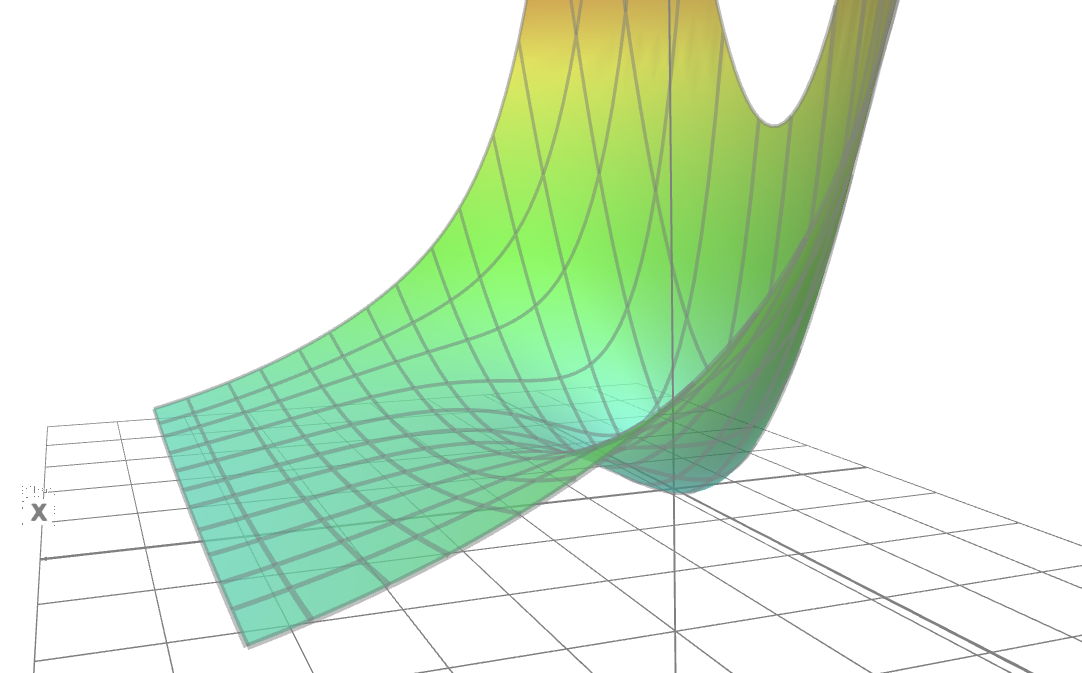
Problem: Consider the function $f$:

$$f(x,y)=(x^2+y^2)e^{-x}.$$

Determine the local extrema of $f$ by finding and analyzing its critical points.

Solution: We set $f_x=0,f_y=0$ and solve this system of equations for points $(x,y)$. By computing the partials, we obtain:

$$\begin{array}{rl}(2x-x^2-y^2)e^{-x}& =0\\ 2y{e}^{-x}& =0.\end{array}$$

The second equation implies $y=0$ because $e^{-x}$ is never zero. Plugging this fact into the first equation gives $x(2-x)e^{-x}=0$ which implies $x=0,2$. So the critical points as given by components are $(0,0)$ and $(2,0)$.

Now let us analyze these critical points using the discriminant. Compute:

$$\begin{array}{rl}{f}_{xx}& =(2-4x+x^2+y^2)e^{-x}\\ f_{yy}& =2e^{-x}\\ f_{xy}& =-2y{e}^{-x}.\end{array}$$

Therefore $D(x,y)=2(2-4x+x^2-y^2)e^{-2x}$, and in particular $D(0,0)=4$, $D(2,0)=-4e^{-4}$. We also need $f_{xx}(0,0)=2>0$ and $f_{xx}(2,0)=-2e^{-2}<0$. The discriminant test concludes that $(0,0)$ is a local minimum, while $(2,0)$ is a saddle point.

3D plot: https://www.math3d.org/cDHxQockR

Also try Desmos3d: https://www.desmos.com/3d/17d5d68086

Link to original

Exercise

02

Analyze two critical points

Let $f(x,y)=2x^2-8xy+y^4-4y^3$. Find the two critical points of $f$ and analyze them using the discriminant test. You are encouraged to check your results by graphing the function in Demos3d or Math3d. What is the minimum value taken by $f$?

Link to original

Exercise

03

Maximum on closed domain

Find the global maximum value of $y^2+xy-x^2$ on the square $x\in [0,2]$, $y\in [0,2]$. Where does this occur? Remember to check critical points on the interior and optimize the function on the boundary.

Link to original

Example

Minimal distance

Minimal distance

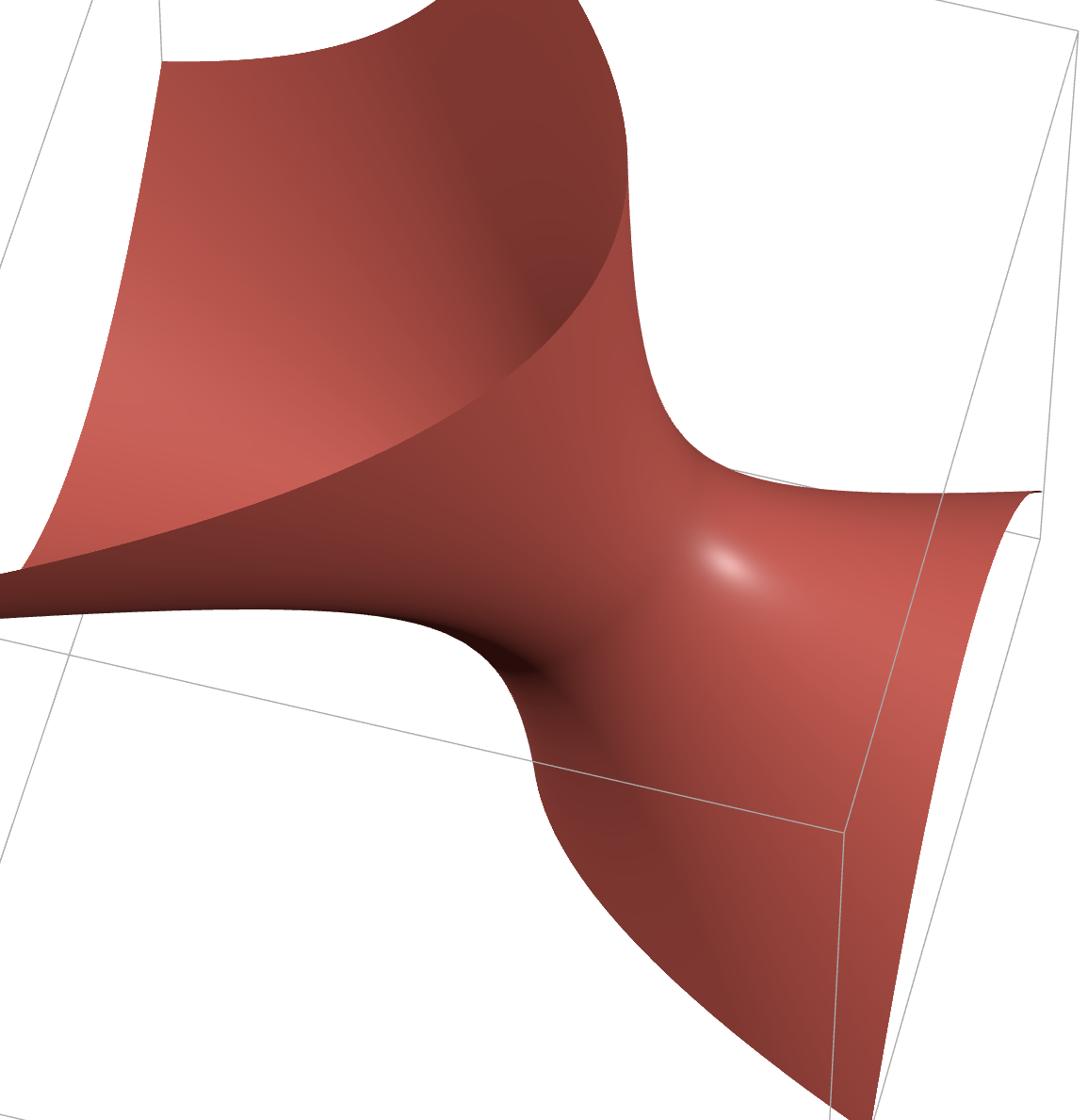
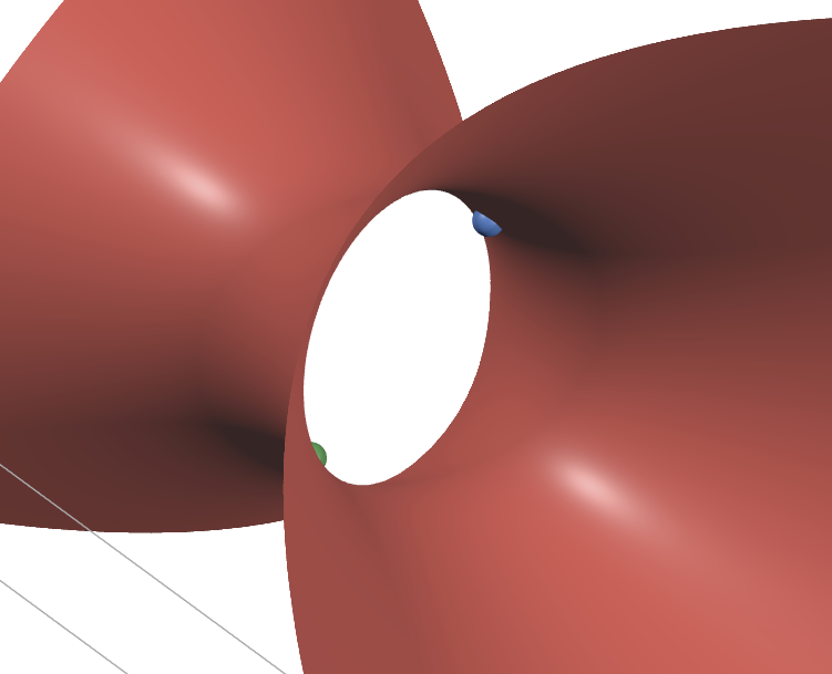
Problem: Consider the surface given by points with coordinates satisfying $y^2=9+xz$. Find the point(s) $(x,y,z)$ closest to the origin.

Solution: Our goal is to extremize the distance to the origin of an arbitrary point on the surface. The distance formula gives $d=\sqrt{x^2+y^2+z^2}$. This function will be extremized at the same place(s) that the function $d^{\prime }=x^2+y^2+z^2$ is extremized because $\sqrt{-}$ is monotone increasing for positive inputs. So we minimize $d^{\prime }$ instead. Next we write the distance as a function of just two variables. Using the surface equation to determine $y^2$, we write $d^{\prime }=9+xz+x^2+z^2$. Then:

$$\begin{array}{rl}{d}_x^{\prime }& =z+2x\\ d_z^{\prime }& =x+2z.\end{array}$$

Setting these simultaneously to zero and solving gives $(x,z)=(0,0)$, and $(x,y,z)$ is $(0,3,0)$ or $(0,-3,0)$. The distance at these points is 3.

Link to original

Exercise

04

Biggest box

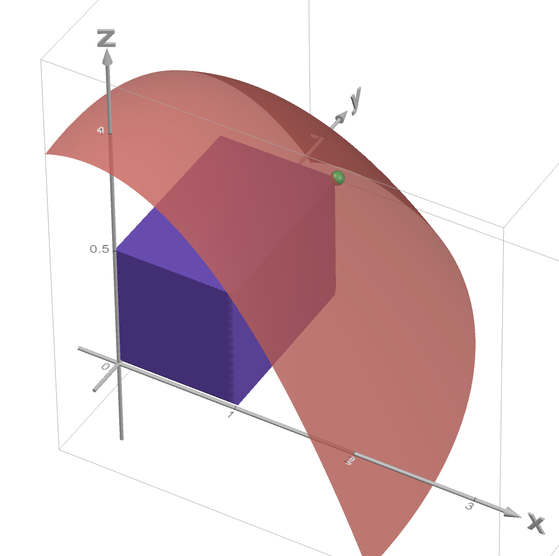
Find the largest volume of a box with nonnegative coordinates, all but one vertex on the coordinate planes, and the remaining vertex lying in the paraboloid given by $\frac{x^2}{4}+\frac{y^2}{9}+z=1$. (So one corner is at the origin, and the opposite corner is on the paraboloid.) What are the dimensions of this box?

Link to original

nD theory

nD theory

(The technique for $n$D requires knowledge of linear algebra, so the next discussion will not be tested in this course.)

In 3D, the same argument about trace curves shows that where $\nabla f=(f_x,f_y,f_z)$ is a non-zero vector, there $f$ is not a local extremum. At such a point, motion in the direction of $\nabla f$ will increase the value of $f$, and motion in the (opposite) direction of $-\nabla f$ will decrease the value of $f$.

Similarly, in $n$D one defines critical points as those points $p$ where $\nabla f(p)$ is either $\vec{0}$ or undefined. Local extrema of $f(x_1,\dots ,x_n)$ can only occur at critical points.

The matrix of second-order partials has a general form called the Hessian matrix:

$$H(x_1,\dots ,x_n)=\left(\begin{array}{ccc}{f}_{x_1{x}_1}& \dots & f_{x_1{x}_n}\\ \dots & \dots & \dots \\ f_{x_n{x}_1}& \dots & f_{x_n{x}_n}\end{array}\right).$$

In 3D the Hessian matrix looks like this:

$$H(x,y,z)=\left(\begin{array}{ccc}{f}_{xx}& f_{xy}& f_{xz}\\ f_{yx}& f_{yy}& f_{yz}\\ f_{zx}& f_{zy}& f_{zz}\end{array}\right).$$

In order to use $H(x,y,z)$ to classify critical points, you have to compute its eigenvalues and count the number of positive and number of negative eigenvalues. (All positive $⇝$ minimum, all negative $⇝$ maximum, various signs $⇝$ saddle.) The determinant is the product of the eigenvalues, so in the 2D theory the discriminant reveals whether the eigenvalues have the same or opposite signs. This explains the discriminant rule that is used in 2D.

Link to original

Constrained optimization: Lagrange multipliers

Introduction

The setup is a function $f(x,y)$ and a curve $\mathcal{C}$. The problem is to find the extremal values of $f(x,y)$ on the curve. If the curve $\mathcal{C}$ is given with a parametrization $\mathbf{r}(t)$, then we could just extremize $f(\mathbf{r}(t))$ using the 1D theory. If the curve is instead given by a constraint such as $g(x,y)=0$, then there is another technique that can be much easier to implement than finding a parametrization $\mathbf{r}(t)$ for $\mathcal{C}$. It is called Lagrange multipliers. Since the constraint is written as $g(x,y)=0$, you can think of this as a relative of implicit differentiation.

The method of Lagrange multipliers makes use of the fact that when $f(x,y)$ is extremized at $p$ on $g(x,y)=0$, then the gradients must align: $\nabla f(p)=\lambda \nabla g(p)$ for some scalar $\lambda$.

Gradients align at extremal values

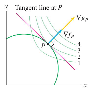
The constraint curve $\mathcal{C}$ is given as the level curve $g(x,y)=c$ with $c=0$. To show the gradients align, we show that they are both perpendicular to this level curve.
Let $\mathbf{r}(t)$ be a parametrization of $\mathcal{C}$. We have already seen that:

$$0=\frac{d}{dt}0=\frac{d}{dt}g(\mathbf{r}(t))=\nabla g\cdot {\mathbf{r}}^{\prime }(t)$$

for any $t$, so $\nabla g$ is always perpendicular to the level curves. In addition, at the specific time $t_0$ where $f(\mathbf{r}(t))$ is extremized, we also have from the 1D optimization theory and the chain rule:

$$0={\frac{d}{dt}f(\mathbf{r}(t))|}_{t_0}=\nabla f(\mathbf{r}(t_0))\cdot {\mathbf{r}}^{\prime }(t_0),$$

and this shows that $\nabla f$ is also perpendicular to the level curve $g(x,y)=0$ at $t_0$. Since both are perpendicular to the level curve, they must point along the same line.

Lagrange multipliers: parallel level curves

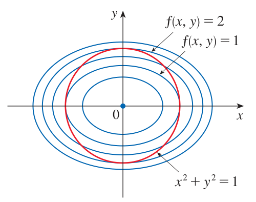
It is convenient to visualize the Lagrange condition on a contour map. The curve $\mathcal{C}$ will be parallel to the level curves of $f(x,y)$ at the points where the value of $f(x,y)$ is extremized on $\mathcal{C}$.

If the level curves of $f$ are not parallel to $\mathcal{C}$ at a point $p$, then it is possible to increase or decrease $f$ by moving along $\mathcal{C}$ because this motion will cross over level curves of $f$.

Because $\mathcal{C}$ is a level curve of $g(x,y)$, it is perpendicular to $\nabla g$. So the level curves of $g$ and $f$ must be parallel at an extremal point. This happens if and only if the gradients are parallel.

Link to original

Example

Lagrange multipliers

Lagrange multipliers

Problem: Find the extreme values of $f(x,y,z)=3x+2y+4z$ on the ellipsoid $x^2+2y^2+6z^2=1$.
Solution: We define $g(x,y,z)=x^2+2y^2+6z^2$. Write out the Lagrange Equations:

$$\nabla f=(3,2,4),\nabla g=(2x,4y,12z),(3,2,4)=\lambda (2x,4y,12z).$$

Solve the system of equations by first solving for $\lambda$ in each coordinate and then equating these values:

$$\frac{3}{2}=\lambda x,\frac{1}{2}=\lambda y,\frac{1}{3}=\lambda z.$$

Obtain $x=\frac{9}{2}z$ and $y=\frac{3}{2}z$. Insert these expressions into the equation $g(x,y,z)=1$ and find a single equation, the solutions of which are $z_p=\frac{2}{\sqrt{123}}$ and $z_q=\frac{-2}{\sqrt{123}}$. Using these expressions again, we find the other coordinates of two critical points:

$$p=\frac{1}{\sqrt{123}}(9,3,2),q=-\frac{1}{\sqrt{123}}(9,3,2).$$

Plug these points into $f(x,y,z)$ and obtain $f(p)=\sqrt{\frac{41}{3}}$ and $f(q)=-\sqrt{\frac{41}{3}}$.

Since the ellipsoid has no boundary, these are the global max and min of $f$ on the ellipsoid.

Link to original

Exercise

01

Lagrange multipliers

Find the extreme values taken by the function on the curve that is given by the equation:

• (a) $f(x,y)=x^2-y^2$, $x^2+y^2=1$
• (b) $f(x,y)=xy{e}^{-x^2-y^2}$, $2x-y=0$

Link to original